Calculate and plot smoothed time series.

Plot time series smoothed by discrete symmetric smoothing kernels. These kernels can be used to smooth time series objects. Options include moving averages, triangular filters, or approximately Gaussian filters.

panel.tskernel(x, y, ...,
    width = NROW(x) %/% 10 + 1, n = 300,
    c = 1, sides = 2, circular = FALSE,
    kern = kernel("daniell",
           rep(floor((width/sides) / sqrt(c)), c)))

simpleSmoothTs(x, ...)

# Default S3 method
simpleSmoothTs(x, ...,
    width = NROW(x) %/% 10 + 1, n = NROW(x),
    c = 1, sides = 2, circular = FALSE,
    kern = kernel("daniell",
           rep(floor((width/sides)/sqrt(c)), c)))

# S3 method for class 'zoo'
simpleSmoothTs(x, ..., n = NROW(x))

Arguments

x, y

data points. Should define a regular, ordered series. A time series object can be passed as the first argument, in which case y can be omitted. The x argument given to simpleSmoothTs is allowed to be a multivariate time series, i.e. to have multiple columns.

...

further arguments passed on to panel.lines.

width

nominal width of the smoothing kernel in time steps. In the default case, which is a simple moving average, this is the actual width. When c > 1 the number of time steps used in the kernel increases but the equivalent bandwidth stays the same. If only past values are used (with sides = 1) then width refers to one side of the symmetric kernel.

n

approximate number of time steps desired for the result. If this is less than the length of x, the smoothed time series will be aggregated by averaging blocks of (an integer number of) time steps, and this aggregated series will be centered with respect to the original series.

c

smoothness of the kernel: c = 1 is a moving average, c = 2 is a triangular kernel, c = 3 and higher approximate smooth Gaussian kernels. c is actually the number of times to recursively convolve a simple moving average kernel with itself. The kernel size is adjusted to maintain a constant equivalent bandwidth as c increases.

sides

if sides=1 the smoothed series is calculed from past values only (using one half of the symmetric kernel); if sides=2 it is centred around lag 0.

circular

to treat the data as circular (periodic).

kern

a tskernel object; if given, this over-rides width and c.

Note

The author is not an expert on time series theory.

Author

Felix Andrews felix@nfrac.org

See also

kernel, filter, xyplot.ts

Examples

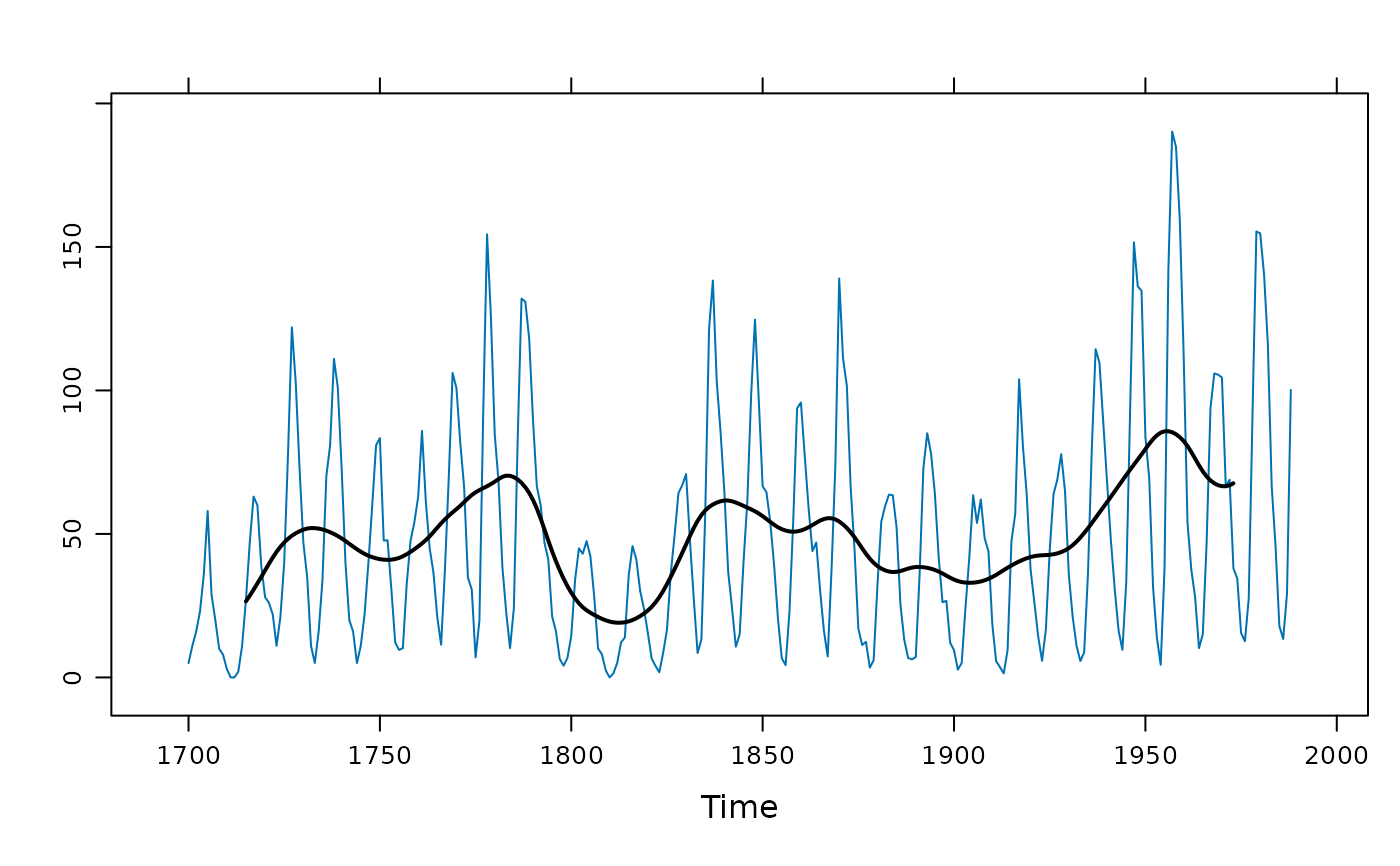
## a Gaussian-like filter (contrast with c = 1 or c = 2)
xyplot(sunspot.year) +
layer(panel.tskernel(x, y, width = 20, c = 3, col = 1, lwd = 2))


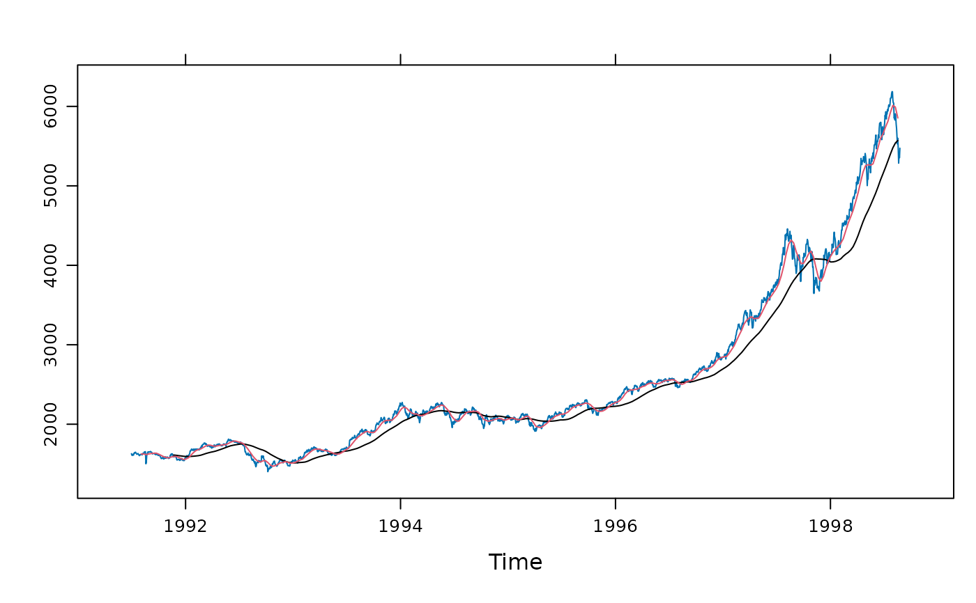
## example from ?kernel:
## long and short moving averages, backwards in time
xyplot(EuStockMarkets[,1]) +
  layer(panel.tskernel(x, y, width = 100, col = 1, sides = 1)) +
  layer(panel.tskernel(x, y, width = 20, col = 2, sides = 1))


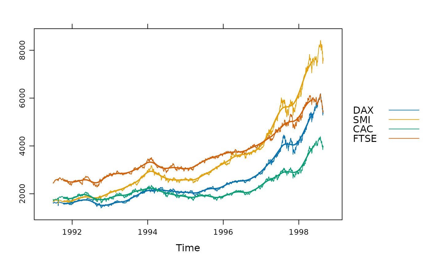
## per group, with a triangular filter
xyplot(EuStockMarkets, superpose = TRUE) +
  glayer(panel.tskernel(..., width = 100, c = 2),
         theme = simpleTheme(lwd = 2))


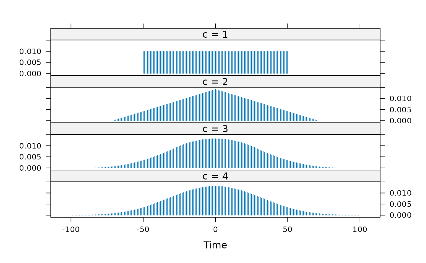
## plot the actual kernels used; note adjustment of width
width = 100
kdat <- lapply(1:4, function(c) {
    k <- kernel("daniell", rep(floor(0.5*width / sqrt(c)), c))
    ## demonstrate that the effective bandwidth stays the same:
    message("c = ", c, ": effective bandwidth = ", bandwidth.kernel(k))
    ## represent the kernel as a time series, for plotting
    ts(k[-k$m:k$m], start = -k$m)
})
#> c = 1: effective bandwidth = 29.1561885940761
#> c = 2: effective bandwidth = 28.9841910933069
#> c = 3: effective bandwidth = 28.4970758733828
#> c = 4: effective bandwidth = 29.440618200031
names(kdat) <- paste("c =", 1:4)
xyplot(do.call(ts.union, kdat), type = "h",
    scales = list(y = list(relation = "same")))