The Art of Influence

A Practical Guide to Working with Influence Functions

Klaus Kähler Holst

2026-08-28

Influence functions

Estimators that have parametric convergence rates can often be fully characterized by their influence function (IF), also referred to as an influence curve (Bickel et al. 1998; Vaart 1998). The IF allows for the direct estimation of properties of the estimator, including its asymptotic variance. Moreover, estimates of the IF enable the simple combination and transformation of estimators into new ones. This vignette describes how to estimate and manipulate IFs using the R-package lava (Holst and Budtz-Jørgensen 2013).

Formally, let $Z_1,\ldots,Z_n$ be iid $k$-dimensional stochastic variables, $Z_i=(Y_{i},A_{i},W_{i})\sim P_{0}$, and $\widehat{\theta}$ a consistent estimator for the parameter $\theta\in\mathbb{R}^p$. When $\widehat{\theta}$ is a regular and asymptotic linear (RAL) estimator, it has a unique iid decomposition $$\begin{align*} \sqrt{n}(\widehat{\theta}-\theta) = \frac{1}{\sqrt{n}}\sum_{i=1}^n \operatorname{IC}(Z_i; P_{0}) + o_{P}(1), \end{align*}$$ where the function $\operatorname{IC}$ is the unique Influence Function s.t. $\mathbb{E}\{\operatorname{IC}(Z_{i}; P_{0})\}=0$ and $\mathbb{V}\!\text{ar}\{\operatorname{IC}(Z_{i}; P_{0})\}<\infty$(Tsiatis 2006; Vaart 1998). The influence function thus fully characterizes the asymptotic behaviour of the estimator and by the central limit theorem it follows that the estimator converges weakly to a Gaussian distribution $$\sqrt{n}(\widehat{\theta}-\theta) \overset{\mathcal{D}}{\longrightarrow} \mathcal{N}(0, \mathbb{V}\!\text{ar}\{\operatorname{IC}(Z; P_{0})\}),$$ where the empirical variance of the plugin estimator, $\mathbb{P}_{n}\operatorname{IC}(Z; \widehat{P})^{\otimes 2} = \frac{1}{n}\sum_{i=1}^n \operatorname{IC}(Z_{i}; \widehat{P})\operatorname{IC}(Z_{i}; \widehat{P})^{\top}$ can be used to obtain a consistent estimate of the asymptotic variance. Note, in practice the estimate $\widehat{P}$ used in the plugin-estimate, needs only to capture the parts of the distribution of $Z$ that is necessary to evaluate the IF. In some cases this nuisance parameter can be estimated using flexible machine learning components and in other (parametric) cases be derived directly from $\widehat{\theta}$.

The IFs are easily derived for the parameters of many parametric statistical models as illustrated in the next example sections. More generally, the IF can also be derived for a smooth target parameter $\Psi: \mathcal{P}\to\mathbb{R}$ where $\mathcal{P}$ is a family of probability distributions forming the statistical model, which often can be left completely non-parametric. Formally, the parameter must be pathwise differentiable see (Vaart 1998) in the sense that there exists a bounded linear functional $\dot\Psi\colon L_{2}(P_{0})\to\mathbb{R}$ such that $[\Psi(P_{t}) - \Psi(P_{0})]t^{-1} \to \dot\Psi(P_{0})(g)$ as $t\to 0$ for any parametric submodel $P_t$ with score model $g(z)= \partial/(\partial t) \log (p_t)(z)|_{t=0}$. Riesz’s representation theorem then tells us that the directional derivative has a unique representer, $\phi_{P_{0}}$ lying in the closure of the submodel score space (the tangent space), s.t. $$\begin{align*} \dot\Psi(P_0)(g) = \langle\phi_{P_0}, g\rangle = \int \phi_{P_0}(z)g(z)\,dP_0(z) \end{align*}$$ The unique representer is exactly the IF which can be found by solving the above integral equation. For more details on how to derive influence functions, we refer to (Laan and Rose 2011; Hines et al. 2022).

As an example we might be interested in the target parameter $\Psi(P) = \mathbb{E}_P(Z)$ which can be shown to have the unique (and thereby efficient) influence function $Z\mapsto Z-\mathbb{E}_P(Z)$ under the non-parametric model. Another target parameter could be $\Psi_{a}(P) = \mathbb{E}_{P}[\mathbb{E}_{P}(Y\mid A=a, W)]$ which is often a key interest in causal inference and which has the IF $$\begin{align*} \operatorname{IC}(Y,A,W; P) = \frac{\mathbf{1}(A=a)}{\mathbb{P}(A=a\mid W)}(Y-\mathbb{E}_{P}[Y\mid A=a,W]) + \mathbb{E}_{P}[Y\mid A=a,W] - \Psi_{a}(P) \end{align*}$$ See section on average treatment effects.

Working with influence functions with lava::estimate

The main functions for working with influence functions are

• estimate which prepares a model object and estimates the IF and corresponding robust standard errors. Can also be used to transform model parameters by application of the Delta Theorem.
• merge method for combining estimates via their estimated IFs
• IC, coef, vcov methods to extract the estimated IF, coefficients, and asymptotic covariance matrix
• subset for extracting subset of parameters and IFs
• transform method for transforming parameter estimates
• labels for renaming parameters

The estimate function is the primary tool for obtaining parameter estimates and related information. It returns an object of the class type estimate, which is a general container for holding information about estimated parameters. The estimate function takes as input either a model object (the first argument x), or a parameter vector and corresponding influence function (IF) matrix specified using the coef and IC arguments. If the primary goal is to apply the delta method or test linear hypotheses, it is also possible to provide the asymptotic variance estimate via the vcov argument, without specifying the IC matrix.

estimate(x=, ...)
estimate(coef=, IC=, ...)
estimate(coef=, vcov=, ...)

A typical call could look like

merge(subset(estimate(x), 1), estimate(coef=p, IC=ic, id=id)) |>
  transform(function(x) c(exp(x), exp(x[1]))) |> # parameter transformation
  labels(c("a", "b")) # rename parameters

Direct calculations are also possible, if a and b are estimate objects we can obtain new transformed parameter estimates with the syntax

c(exp(b)^0.5, exp(b * a) / (1 + exp(-b)))

with the necessary derivatives exactly calculated automatically. We refer to section IF building blocks for more details.

Examples

To illustrate the methods we consider data arising from the model $Y_{ij} \sim Bernoulli\{\operatorname{expit}(X_{ij} + A_{i} + W_{i})\}, A_{i} \sim Bernoulli\{\operatorname{expit}(W_{i})\}$ with independent covariates $X_{ij}\sim\mathcal{N}(0,1), W_{i}\sim\mathcal{N}(0,1)$.

m <- lvm() |>
  regression(y1 ~ x1 + a + w) |>
  regression(y2 ~ x2 + a + w) |>
  regression(y3 ~ x3 + a + w) |>
  regression(y4 ~ x4 + a + w) |>
  regression(a ~ w) |>
  distribution(~ y1 + y2 + y3 + y4 + a, value = dist_bernoulli()) |>
  distribution(~id, value = dist_seq(integer = TRUE))

We simulate from the model where $Y_3$ is only observed for half of the subjects

n <- 1e3
dw <- sim(m, n, seed = 1) |>
  transform(y3 = y3 * ifelse(id > n / 2, NA, 1))
Print(dw)
#>      y1 x1      a w         y2 x2       y3 x3      y4 x4        id  
#> 1    1  -0.6265 1  1.1350   1  -0.88615 1   0.7391 0  -1.1346   1   
#> 2    1   0.1836 1  1.1119   1  -1.92225 1   0.3866 1   0.7646   2   
#> 3    1  -0.8356 1 -0.8708   1   1.61970 1   1.2964 1   0.5707   3   
#> 4    1   1.5953 1  0.2107   1   0.51927 0  -0.8036 0  -1.3517   4   
#> 5    0   0.3295 1  0.0694   0  -0.05585 0  -1.6026 0  -2.0299   5   
#> ---                                                                 
#> 996  0  -0.3133 0 -0.008056 0  -0.1868  NA -0.1422 0   0.162547  996
#> 997  1  -0.8807 1  1.033784 1  -0.2294  NA  0.8643 1   0.980737  997
#> 998  1  -0.4193 1 -0.799127 1   1.6302  NA -0.0219 0  -0.692140  998
#> 999  0  -1.4828 1  1.004233 1  -2.1647  NA -0.2647 1  -0.003494  999
#> 1000 1  -0.6973 0 -0.311973 0  -1.0778  NA -0.9133 1   0.171580 1000
## Data in long format
dl <- reshape(dw,
        varying = list(paste0("y",1:4),
                       paste0("x",1:4)),
        v.names=c("y", "x"), direction="long") |>
  na.omit()
dl <- dl[order(dl$id), ]
## dl <- mets::fast.reshape(dw, varying = c("y", "x")) |> na.omit()
Print(dl)
#>        a w      id   time y x        
#> 1.1    1 1.135  1    1    1 -0.6265  
#> 1.2    1 1.135  1    2    1 -0.8861  
#> 1.3    1 1.135  1    3    1  0.7391  
#> 1.4    1 1.135  1    4    0 -1.1346  
#> 2.1    1 1.112  2    1    1  0.1836  
#> ---                                  
#> 999.2  1  1.004  999 2    1 -2.164671
#> 999.4  1  1.004  999 4    1 -0.003494
#> 1000.1 0 -0.312 1000 1    1 -0.697318
#> 1000.2 0 -0.312 1000 2    0 -1.077776
#> 1000.4 0 -0.312 1000 4    1  0.171580

Example: population mean

Here we first consider the problem of estimating the IF of the mean. For a general transformation $f: \mathbb{R}^k\to\mathbb{R}^p$ we have that $$\sqrt{n}\{\mathbb{P}_{n}f(X) - \mathbb{E}[f(X)]\} = \frac{1}{\sqrt{n}}\sum_{i=1}^{n} \{f(X_{i}) - \mathbb{E}[f(X)]\}$$ and hence for the problem of estimating the proportion of the binary outcome $Y_1$, the IF is given by $\mathbf{1}(Y_{1}=1) - \mathbb{P}(Y_{1}=1)$.

To estimate this parameter and its IF we will use the estimate function

inp <- as.matrix(dw[, c("y1", "y2")])
e <- estimate(inp[, 1, drop = FALSE], type="mean")
class(e)
#> [1] "estimate"
e
#>    Estimate Std.Err   2.5%  97.5%    P-value
#> y1    0.565 0.01568 0.5343 0.5957 2.009e-284

The reported standard errors from the estimate method are the robust standard errors obtained from the IF. The variance estimate and the parameters can be extracted with the vcov and coef methods. The IF itself can be extracted with the IC (or influence) method:

IC(e) |> Print()
#>      y1    
#> 1     0.435
#> 2     0.435
#> 3     0.435
#> 4     0.435
#> 5    -0.565
#> ---        
#> 996  -0.565
#> 997   0.435
#> 998   0.435
#> 999  -0.565
#> 1000  0.435

It is also possible to simultaneously estimate the proportions of each of the two binary outcomes

estimate(inp)
#>    Estimate Std.Err   2.5%  97.5%    P-value
#> y1    0.565 0.01568 0.5343 0.5957 2.009e-284
#> y2    0.560 0.01570 0.5292 0.5908 9.550e-279

or alternatively the input can be a model object, here a mlm object:

e <- lm(cbind(y1, y2) ~ 1, data = dw) |>
  estimate()
IC(e) |> head()
#>   y1:(Intercept) y2:(Intercept)
#> 1          0.435           0.44
#> 2          0.435           0.44
#> 3          0.435           0.44
#> 4          0.435           0.44
#> 5         -0.565          -0.56
#> 6         -0.565           0.44

Different methods are available for inspecting an estimate object

summary(e)
#> Call: estimate.default(x = x, coef = pars(x))
#> ────────────────────────────────────────────────────────────
#>                Estimate Std.Err   2.5%  97.5%    P-value
#> y1:(Intercept)    0.565 0.01568 0.5343 0.5957 2.009e-284
#> y2:(Intercept)    0.560 0.01570 0.5292 0.5908 9.550e-279
#> ────────────────────────────────────────────────────────────
#> Null Hypothesis: 
#>   [y1:(Intercept)] = 0
#>   [y2:(Intercept)] = 0 
#>  
#> chisq = 2056.775, df = 2, p-value < 2.2e-16
## extract parameter coefficients
coef(e)
#> y1:(Intercept) y2:(Intercept) 
#>          0.565          0.560
## ## Asymptotic (robust) variance estimate
vcov(e)
#>                y1:(Intercept) y2:(Intercept)
#> y1:(Intercept)    0.000245775      0.0000616
#> y2:(Intercept)    0.000061600      0.0002464
## Matrix with estimates and confidence limits
summary(e, level = 0.99) |> parameter()
#>                Estimate    Std.Err      0.5%     99.5%       P-value
#> y1:(Intercept)    0.565 0.01567721 0.5246182 0.6053818 2.009130e-284
#> y2:(Intercept)    0.560 0.01569713 0.5195669 0.6004331 9.550279e-279
## Influence curve
IC(e) |> head()
#>   y1:(Intercept) y2:(Intercept)
#> 1          0.435           0.44
#> 2          0.435           0.44
#> 3          0.435           0.44
#> 4          0.435           0.44
#> 5         -0.565          -0.56
#> 6         -0.565           0.44
## Join estimates
ee <- merge(e, e)
ee
#>                  Estimate Std.Err   2.5%  97.5%    P-value
#> y1:(Intercept)      0.565 0.01568 0.5343 0.5957 2.009e-284
#> y2:(Intercept)      0.560 0.01570 0.5292 0.5908 9.550e-279
#> y1:(Intercept).1    0.565 0.01568 0.5343 0.5957 2.009e-284
#> y2:(Intercept).1    0.560 0.01570 0.5292 0.5908 9.550e-279
## Forest plots
plot(ee, null=0.5, digits=2)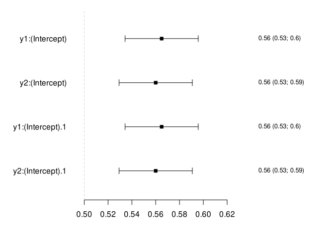

Example: generalized linear model

For a $Z$-estimator defined by the score equation $E[U(Z; \theta)] = 0$, the IF is given by $$\begin{align*} IC(Z; \theta) = -\mathbb{E}\Big\{\frac{\partial}{\partial\theta^\top}U(\theta; Z)\Big\}^{-1}U(Z; \theta) \end{align*}$$ In particular, for a maximum likelihood estimator the score, $U$, is given by the partial derivative of the log-likelihood function.

As an example, we can obtain the estimates with robust standard errors for a logistic regression model:

g <- glm(y1 ~ a + x1, data = dw, family = binomial)
estimate(g)
#>             Estimate Std.Err    2.5%   97.5%   P-value
#> (Intercept)  -0.4033 0.09781 -0.5950 -0.2116 3.742e-05
#> a             1.5832 0.15030  1.2886  1.8778 6.052e-26
#> x1            0.8837 0.08061  0.7257  1.0417 5.835e-28

We can compare that to the usual (non-robust) standard errors by supplying the model-based covariance matrix explicitly:

estimate(g, vcov = vcov(g))
#>             Estimate Std.Err    2.5%   97.5%   P-value
#> (Intercept)  -0.4033 0.09682 -0.5930 -0.2135 3.111e-05
#> a             1.5832 0.15138  1.2865  1.8799 1.335e-25
#> x1            0.8837 0.08231  0.7223  1.0450 6.904e-27
# estimate(g, vcov = TRUE) alternative syntax to obtain model-based SEs

The IF can be extracted from the estimate object or directly from the model object

IC(g) |> head()
#>   (Intercept)          a         x1
#> 1  0.07717226   4.001259 -0.7195347
#> 2 -0.07604185   2.866943  0.7089951
#> 3  0.14619472   4.257845 -1.3630828
#> 4 -0.09723106   1.252449  0.9065580
#> 5  0.38472247 -11.599820 -3.5870556
#> 6 -2.43751385   2.931614  1.5365778

The same estimates can be obtained with a cumulative link regression model which also generalizes to ordinal outcomes. Here we consider the proportional odds model given by $$\begin{align*} \log\left(\frac{\mathbb{P}(Y\leq j\mid x)}{1-\mathbb{P}(Y\leq j\mid x)}\right) = \operatorname{expit}(\alpha_{j} - \beta^{t}), \quad j=1,\ldots,J-1 \end{align*}$$

ordreg(y1 ~ a + x1, dw, family=binomial(logit)) |> estimate()
#>     Estimate Std.Err   2.5% 97.5%   P-value
#> 0|1   0.4033 0.09781 0.2116 0.595 3.743e-05
#> a     1.5832 0.15031 1.2886 1.878 6.080e-26
#> x1    0.8837 0.08062 0.7257 1.042 5.866e-28

Note that the sandwich::estfun function from the sandwich library (Zeileis et al. 2020) can also be used to estimate the IF for different parametric models, but does not provide the tools for combining and transforming these.

Example: right-censored outcomes

To illustrate the methods on survival data we will use the Mayo Clinic Primary Biliary Cholangitis Data (Therneau and Grambsch 2000)

library("survival")
data(pbc, package="survival")

The Cox proportional hazards model can be fitted with the mets::phreg method which can estimate the IF for both the partial likelihood parameters and the baseline hazard. Here we fit a survival model with right-censored event times

fit.phreg <- mets::phreg(Surv(time, status > 0) ~ age + sex, data = pbc)
fit.phreg
#> Call:
#> mets::phreg(formula = Surv(time, status > 0) ~ age + sex, data = pbc)
#> 
#>    n events
#>  418    186
#> 
#> coefficients:
#>        age       sexf 
#>  0.0220977 -0.2999507
IC(fit.phreg) |> head()
#>           age       sexf
#> 1  0.12691175  2.9551968
#> 2 -0.16011629 -4.3755455
#> 3  0.19322595 -8.1786480
#> 4  0.04668109  0.8548021
#> 5 -0.22936186  0.9721761
#> 6  0.07015171  0.5644414

The IF for the baseline cumulative hazard at a specific time point $$\begin{align*} \Lambda_0(t) = \int_0^t \lambda_0(u)\,du, \end{align*}$$ where $\lambda_0(t)$ is the baseline hazard, can be estimated in similar way:

baseline <- function(object, time, ...) {
  ic <- mets::IC(object, baseline = TRUE, time = time, ...)
  est <- mets::predictCumhaz(object$cumhaz, new.time = time)[1, 2]
  estimate(NULL, coef = est, IC = ic, labels = paste0("chaz:", time))
}
tt <- 2000
baseline(fit.phreg, tt)
#>           Estimate Std.Err    2.5%  97.5% P-value
#> chaz:2000    0.178 0.07597 0.02913 0.3269 0.01911

The estimate and IC methods are also available for parametric survival models via survival::survreg, here a Weibull model:

survival::survreg(Surv(time, status > 0) ~ age + sex, data = pbc, dist="weibull") |>
  estimate()
#>             Estimate  Std.Err     2.5%     97.5%    P-value
#> (Intercept)  9.02697 0.382437  8.27741  9.776530 3.521e-123
#> age         -0.01919 0.006362 -0.03166 -0.006723  2.554e-03
#> sexf         0.28170 0.174338 -0.06000  0.623392  1.061e-01
#> scale        0.87751 0.070693  0.73896  1.016067  2.220e-35

Example: random effects model / structural equation model

General structural equation models (SEMs) can be estimated with lava::lvm. Here we fit a random effects probit model $$\mathbb{P}(Y_{ij} = 1 \mid U_{i}, W_{ij})=\Phi(\mu_{j} + \beta_{j} W_{ij} + U_{i}), \quad U_{i}\sim\mathcal{N}(0,\sigma_{u}^{2}),\quad j=1,2$$ to the simulated dataset

sem <- lvm(y1 + y2 ~ 1 * u + w) |>
  latent(~ u) |>
  ordinal(K=2, ~ y1 + y2)
semfit <- estimate(sem, data = dw)

## Robust standard errors
estimate(semfit)
#>      Estimate Std.Err     2.5%  97.5%   P-value
#> y2   -0.01236 0.06232 -0.13450 0.1098 8.428e-01
#> u     0.21656 0.04640  0.12562 0.3075 3.052e-06
#> y1~w  0.59037 0.05307  0.48635 0.6944 9.645e-29
#> y2~w  0.65419 0.05599  0.54446 0.7639 1.528e-31
#> u~~u  0.19001 0.07614  0.04078 0.3392 1.257e-02

Example: quantile

Let $\beta$ denote the $\tau$th quantile of $X$, with IF $$\begin{align*} \operatorname{IC}(x; P_{0}) = \{\tau - \mathbf{1}(x\leq \beta)\}f_{0}(\beta)^{-1} \end{align*}$$

where $f_{0}$ is the density function of $X$.

To calculate the variance estimate, an estimate of the density is thus needed which can be obtained by a kernel estimate. Alternatively, the resampling method of (Zeng and Lin 2008) can be applied. Here we use a kernel smoother (additional arguments to the estimate function are parsed on to stats::density.default) to estimate the quantiles and IF for the 25%, 50%, and 75% quantiles of $W$ and $X_1$

eq <- estimate(dw[, c("w", "x1")], type = "quantile", probs = c(0.25, 0.5, 0.75))
eq
#>        Estimate Std.Err    2.5%    97.5%   P-value
#> w.25%  -0.68967 0.04493 -0.7777 -0.60161 3.465e-53
#> w.50%  -0.03448 0.04091 -0.1147  0.04570 3.993e-01
#> w.75%   0.73734 0.04784  0.6436  0.83111 1.354e-53
#> x1.25% -0.69737 0.04586 -0.7873 -0.60749 3.172e-52
#> x1.50% -0.03532 0.04176 -0.1172  0.04653 3.977e-01
#> x1.75%  0.68843 0.04366  0.6029  0.77400 5.246e-56
IC(eq) |> head()
#>           w.25%     w.50%      w.75%     x1.25%    x1.50%     x1.75%
#> [1,]  0.8202184  1.293737  2.6203624  0.8372545 -1.320712 -0.7971649
#> [2,]  0.8202184  1.293737  2.6203624  0.8372545  1.320712 -0.7971649
#> [3,] -2.4606551 -1.293737 -0.8734541 -2.5117634 -1.320712 -0.7971649
#> [4,]  0.8202184  1.293737 -0.8734541  0.8372545  1.320712  2.3914946
#> [5,]  0.8202184  1.293737 -0.8734541  0.8372545  1.320712 -0.7971649
#> [6,] -2.4606551 -1.293737 -0.8734541 -2.5117634 -1.320712 -0.7971649

Combining influence functions

A key benefit of working with the IFs of estimators is that this allows for transforming or combining different estimates while easily deriving the resulting IF and thereby asymptotic distribution of the new estimator.

Lemma 1 Let $\widehat{\theta}_{1}, \ldots, \widehat{\theta}_{M}$ be $M$ different estimators with decompositions $$\begin{align*} \sqrt{n}(\widehat{\theta}_{m}-\theta_{m}) = \frac{1}{\sqrt{n}}\sum_{i=1}^{n} \operatorname{IC}_m(Z_i; P_{0}) + o_{P}(1) \end{align*}$$ based on iid data $Z_1,\ldots,Z_n$. Then the joint estimate $\widehat{\theta} = (\widehat{\theta}_{1}^{\top},\ldots,\widehat{\theta}_{M}^{\top})^\top$ of ${\theta} = ({\theta}_{1}^{\top},\ldots,{\theta}_{M}^{\top})^\top$ has influence function given by $$\begin{align*} \overline{\operatorname{IC}}(Z_i; P_{0}) = [\operatorname{IC}_{1}(Z_i; P_{0})^\top,\ldots,\operatorname{IC}_{M}(Z_i; P_{0})^\top]^{\top}. \end{align*}$$$\blacksquare$

This follows immediately from (Vaart 1998, Theorem 18.10[vi]), and thus $$\begin{align*} \sqrt{n}(\widehat{\theta}-\theta) &= \frac{1}{\sqrt{n}}\sum_{i=1}^{n} \underbrace{[\operatorname{IC}_{1}(Z_i; P_{0})^\top,\ldots,\operatorname{IC}_{M}(Z_i; P_{0})^\top]^{\top}}_{\overline{\operatorname{IC}}(Z_i; P_{0})} + o_{P}(1) \\ &\overset{\mathcal{D}}{\longrightarrow}\mathcal{N}(0,\Sigma) \end{align*}$$ by the CLT, and under regularity conditions $\mathbb{P}_{n}\overline{\operatorname{IC}}(Z_i; \widehat{P})^{\otimes 2} \overset{P}{\longrightarrow}\Sigma$ as $n\to\infty$.

To illustrate this we consider two marginal logistic regression models fitted separately for $Y_1$ and $Y_2$ and combine the estimates and IFs using the merge method

g1 <- glm(y1 ~ a, family=binomial, data=dw)
g2 <- glm(y2 ~ a, family=binomial, data=dw)
e <- merge(g1, g2)
summary(e)
#> Call: estimate.default(data = NULL, id = id, coef = coefs, IC = ic0, 
#>     stack = FALSE, keep = keep)
#> ────────────────────────────────────────────────────────────
#>               Estimate Std.Err    2.5%   97.5%   P-value
#> (Intercept)    -0.3706 0.08887 -0.5448 -0.1964 3.048e-05
#> a               1.4031 0.13692  1.1347  1.6714 1.218e-24
#> (Intercept).1  -0.4342 0.08944 -0.6095 -0.2589 1.207e-06
#> a.1             1.4995 0.13792  1.2291  1.7698 1.562e-27
#> ────────────────────────────────────────────────────────────
#> Null Hypothesis: 
#>   [(Intercept)] = 0
#>   [a] = 0
#>   [(Intercept).1] = 0
#>   [a.1] = 0 
#>  
#> chisq = 214.6624, df = 4, p-value < 2.2e-16

As we have access to the joint asymptotic distribution we can for example test for whether the odds-ratio is the same for the two responses:

summary(estimate(e), contrast=cbind(0,1,0,-1), null=0)
#> Call: estimate.default(x = e)
#> ────────────────────────────────────────────────────────────
#>               Estimate Std.Err    2.5%   97.5%   P-value
#> (Intercept)    -0.3706 0.08887 -0.5448 -0.1964 3.048e-05
#> a               1.4031 0.13692  1.1347  1.6714 1.218e-24
#> (Intercept).1  -0.4342 0.08944 -0.6095 -0.2589 1.207e-06
#> a.1             1.4995 0.13792  1.2291  1.7698 1.562e-27
#> ────────────────────────────────────────────────────────────
#> Null Hypothesis: 
#>   [a] - [a.1] = 0 
#>  
#> chisq = 0.2869, df = 1, p-value = 0.5922

More details can be found in the Section on hypothesis testing.

Estimators computed on different subsets

Let $O_1 = (Z_1, R_1), \ldots, O_N = (Z_N, R_N)$ be iid data from some distribution $O = (Z, R) \sim P_0$. We let $Q_0 := P_0(\cdot \mid R=1)$ denote the conditional distribution, with $P(R=1) = p > 0$, and let $S = \{i\mid R_i=1\}$, $n = \lvert S\rvert$, and $\widehat{p} = n/N$.

We assume that the conditional target parameter $\theta = T(Q_0)$ is pathwise differentiable in $Q_0$, in the sense that we have a regular and asymptotic linear estimator $\widehat{\theta} = T_m(O_1, \ldots, O_m)$ based on iid data $O_1,\ldots,O_m \sim Q_0$, such that for any $\eta>0$$$\begin{align*} g(m, \eta) = Q\Big( \big\lVert \underbrace{ \sqrt{m}\left\{ T_m(O_1, \ldots, O_m) - \theta - \frac{1}{m}\sum_{i=1}^m \operatorname{IC}(O_i; Q_0) \right\} }_{V_m} \big\rVert > \eta \Big) \longrightarrow 0 \text{ as } m\to\infty. \end{align*}$$

Lemma 2 The estimator $\widehat{\theta}$ has influence function $\widetilde{\operatorname{IC}}(O; Q_0) = \frac{R}{p}\operatorname{IC}(O; Q_0)$, i.e. $$\begin{align*} \sqrt{N}(\widehat{\theta} - \theta) = \frac{1}{p}\frac{1}{\sqrt{N}}\sum_{i=1}^N R_i \operatorname{IC}(O_i; Q_0) + o_{P_0}(1). \end{align*}$$

Proof. We can write $$\begin{align*} \sqrt{N}(\widehat{\theta}-\theta) = \frac{1}{\widehat{p}}\frac{1}{\sqrt{N}} \sum_{i=1}^N R_i \operatorname{IC}(O_i; Q_0) + \underbrace{\sqrt{N}\left( \widehat{\theta}-\theta-\frac{1}{n}\sum_{i\in S}\operatorname{IC}(O_i; Q_0) \right)}_{W_N = \sqrt{N/n}V_n}. \end{align*}$$

We need to show that the term $W_N=o_{P_0}(1)$. Let $E_N = \{n > Np/2\}$, it then follows that $$\begin{align*} P(\lVert W_N \rVert > \epsilon) \leq P(E_N^\complement) + P(\{\lVert W_N \rVert > \epsilon\}\cap E_N) \\ \leq P(E_N^\complement) + \sup_{n>Np/2} Q(\lVert V_n \rVert > \epsilon/c) \end{align*}$$ where we have used that on the set $E_N$ we have $\sqrt{N/n}< \sqrt{2/p} = c$. The supremum term converges to zero as $N\to\infty$ due to the assumption that $\widehat{\theta}$ is RAL in $Q_0$.

Applying Hoeffding’s Inequality to the iid Bernoulli random variables $1-R_i, i=1,\ldots,N$, we get that $$\begin{align*} P(N-n - N(1-p) \geq t) \leq \exp(-2t^2/N), \end{align*}$$ and with $t = Np/2$, we have that $P(n<Np/2)\leq\exp(-N/(2p^2))\to 0$ as $N\to\infty$, and it follows that the first term $P(E_N^\complement)$ also converges to zero.

As $\widehat{p}\to p$ a.s. by the strong LLN, it follows from continuity at $p>0$ that $\widehat{p}^{-1}-p^{-1} = o_{P_0}(1)$, and hence by Slutsky’s lemma $$\begin{align*} \sqrt{N}(\widehat{\theta}-\theta) &= \frac{1}{\sqrt{N}}\sum_{i=1}^N \frac{R_i}{p}\operatorname{IC}(O_i; Q_0) + (\frac{1}{\widehat{p}}-\frac{1}{p}) \frac{1}{\sqrt{N}}\sum_{i=1}^N R_i\operatorname{IC}(O_i; Q_0) + o_{P_0}(1) \\ &= \frac{1}{\sqrt{N}}\sum_{i=1}^N \frac{R_i}{p}\operatorname{IC}(O_i; Q_0) + o_{P_0}(1). \end{align*}$$$\blacksquare$

Based on the above Lemma we can therefore combine estimators that are estimated on different datasets. Let the observed data be $(Z_{11}, R_{11}), (Z_{21}, R_{21}), \ldots, (Z_{1N}, R_{1N}), (Z_{2N}, R_{2N})$ with estimators $\widehat{\theta}_1$ and $\widehat{\theta}_2$ for the conditional parameters $\theta_1$ and $\theta_2$ based on data where $R_{1i}=1$ and $R_{2j}=1$, respectively, and let the corresponding IFs be $IC_{1}(\cdot; P_{0})$ and $IC_{2}(\cdot;P_{0})$. It then follows that the joint parameter estimate has influence function corresponding to an inverse probability weighting with the empirical plugin estimate of the proportions $P(R_{1}=1)$, and $P(R_{2}=1)$$$\begin{align*} \sqrt{N}\left\{ \begin{pmatrix} \widehat{\theta}_1 \\ \widehat{\theta}_2 \end{pmatrix} - \begin{pmatrix} \vphantom{\widehat{\theta}_1}\theta_1 \\ \vphantom{\widehat{\theta}_1}\theta_2 \end{pmatrix} \right\} = \frac{1}{\sqrt{N}}\sum_{i=1}^N \begin{pmatrix} IC_1(Z_{1i}; P_{0})\frac{R_{1i}N}{R_{1\bullet}} \\ IC_2(Z_{2i}; P_{0})\frac{R_{2i}N}{R_{2\bullet}} \end{pmatrix} + o_{P}(1) \end{align*}$$

with $R_{k\bullet} = \sum_{i=1}^{N}R_{ki}.$ Returning to the example, we can combine the marginal estimates of two model objects that have been estimated from different datasets (as the outcome $Y_3$ is only available in half of the data) with the merge function

g2 <- glm(y2 ~ 1, family = binomial, data = dw)
summary(g2)
#> 
#> Call:
#> glm(formula = y2 ~ 1, family = binomial, data = dw)
#> 
#> Coefficients:
#>             Estimate Std. Error z value Pr(>|z|)    
#> (Intercept)  0.24116    0.06371   3.786 0.000153 ***
#> ---
#> Signif. codes:  0 '***' 0.001 '**' 0.01 '*' 0.05 '.' 0.1 ' ' 1
#> 
#> (Dispersion parameter for binomial family taken to be 1)
#> 
#>     Null deviance: 1371.9  on 999  degrees of freedom
#> Residual deviance: 1371.9  on 999  degrees of freedom
#> AIC: 1373.9
#> 
#> Number of Fisher Scoring iterations: 3
dwc <- na.omit(dw)
g3 <- glm(y3 ~ 1, family = binomial, data = dwc)
summary(g3)
#> 
#> Call:
#> glm(formula = y3 ~ 1, family = binomial, data = dwc)
#> 
#> Coefficients:
#>             Estimate Std. Error z value Pr(>|z|)    
#> (Intercept)   0.3474     0.0908   3.827  0.00013 ***
#> ---
#> Signif. codes:  0 '***' 0.001 '**' 0.01 '*' 0.05 '.' 0.1 ' ' 1
#> 
#> (Dispersion parameter for binomial family taken to be 1)
#> 
#>     Null deviance: 678.28  on 499  degrees of freedom
#> Residual deviance: 678.28  on 499  degrees of freedom
#> AIC: 680.28
#> 
#> Number of Fisher Scoring iterations: 4

e2 <- estimate(g2, id = dw$id)
e3 <- estimate(g3, id = "id", data=dwc)

ecomb <- merge(e2, e3)
IC(ecomb) |> Print()
#>      (Intercept) (Intercept).1
#> 1     1.786       3.413       
#> 2     1.786       3.413       
#> 3     1.786       3.413       
#> 4     1.786      -4.831       
#> 5    -2.273      -4.831       
#> ---                           
#> 996  -2.273       0.000       
#> 997   1.786       0.000       
#> 998   1.786       0.000       
#> 999   1.786       0.000       
#> 1000 -2.273       0.000
vcov(ecomb)
#>               (Intercept) (Intercept).1
#> (Intercept)   0.004058270   0.001140603
#> (Intercept).1 0.001140603   0.008243887
## Same marginals as
list(vcov(e2), vcov(e3))
#> [[1]]
#>             (Intercept)
#> (Intercept)  0.00405827
#> 
#> [[2]]
#>             (Intercept)
#> (Intercept) 0.008243887

Note, it is also possible to directly specify the id-variables in the merge call:

merge(e2, e3, id = list(dw$id, dwc$id))
#>               Estimate Std.Err   2.5%  97.5%   P-value
#> (Intercept)     0.2412  0.0637 0.1163 0.3660 0.0001533
#> (Intercept).1   0.3475  0.0908 0.1695 0.5254 0.0001298

In the above example the id argument defines the identifier that makes it possible to link the rows in the different IFs that should be glued together. If omitted then the id will automatically be extracted from the model-specific IC method (deriving it from the original data.frame used for estimating the model). This automatically works with all models and IC methods described in this document.

estimate(g2) |>
  IC() |> head()
#>   (Intercept)
#> 1    1.785677
#> 2    1.785677
#> 3    1.785677
#> 4    1.785677
#> 5   -2.272679
#> 6    1.785677
vcov(merge(estimate(g2), estimate(g3)))
#>               (Intercept) (Intercept).1
#> (Intercept)   0.004058270   0.001140603
#> (Intercept).1 0.001140603   0.008243887
merge(estimate(g2), estimate(g3)) |>
  (rownames %++% head %++% IC)()
#> [1] "1" "2" "3" "4" "5" "6"

To force that the id variables are not overlapping between the merged model objects, i.e., assuming that there is complete independence between the estimates, the argument id=NULL can be used

merge(g1, g2, id = NULL) |> (Print %++% IC)()
#>      (Intercept) a          (Intercept).1
#> 1    -5.097e-16   5.698e+00  0.000e+00   
#> 2    -5.097e-16   5.698e+00  0.000e+00   
#> 3    -5.097e-16   5.698e+00  0.000e+00   
#> 4    -5.097e-16   5.698e+00  0.000e+00   
#> 5     3.043e-15  -1.600e+01  0.000e+00   
#> ---                                      
#> 1996  0.000       0.000     -4.545       
#> 1997  0.000       0.000      3.571       
#> 1998  0.000       0.000      3.571       
#> 1999  0.000       0.000      3.571       
#> 2000  0.000       0.000     -4.545
merge(g1, g2, id = NULL) |> vcov()
#>                 (Intercept)             a (Intercept).1
#> (Intercept)    7.898704e-03 -7.898704e-03  4.539224e-28
#> a             -7.898704e-03  1.874767e-02 -2.718185e-24
#> (Intercept).1  4.539224e-28 -2.718185e-24  4.058270e-03

Renaming and subsetting parameters

To only keep a subset of the parameters the keep argument can be used.

merge(g1, g2, keep = c("(Intercept)", "(Intercept).1"))
#>               Estimate Std.Err    2.5%   97.5%   P-value
#> (Intercept)    -0.3706 0.08887 -0.5448 -0.1964 3.048e-05
#> (Intercept).1   0.2412 0.06370  0.1163  0.3660 1.533e-04

The argument can be given either as character vector or a vector of indices:

merge(g1, g2, keep=c(1, 3))
#>               Estimate Std.Err    2.5%   97.5%   P-value
#> (Intercept)    -0.3706 0.08887 -0.5448 -0.1964 3.048e-05
#> (Intercept).1   0.2412 0.06370  0.1163  0.3660 1.533e-04

or as a vector of perl-style regular expressions

merge(g1, g2, keep = "cept", regex = TRUE)
#>               Estimate Std.Err    2.5%   97.5%   P-value
#> (Intercept)    -0.3706 0.08887 -0.5448 -0.1964 3.048e-05
#> (Intercept).1   0.2412 0.06370  0.1163  0.3660 1.533e-04
merge(g1, g2, keep = c("\\)$", "^a$"), regex = TRUE, ignore.case = TRUE)
#>             Estimate Std.Err    2.5%   97.5%   P-value
#> (Intercept)  -0.3706 0.08887 -0.5448 -0.1964 3.048e-05
#> a             1.4031 0.13692  1.1347  1.6714 1.218e-24

When merging estimates unique parameter names are created. It is also possible to rename the parameters with the labels argument

merge(g1, g2, labels = c("a", "b", "c")) |> estimate(keep = c("a", "c"))
#>   Estimate Std.Err    2.5%   97.5%   P-value
#> a  -0.3706 0.08887 -0.5448 -0.1964 3.048e-05
#> c   0.2412 0.06370  0.1163  0.3660 1.533e-04
merge(g1, g2,
      labels = c("a", "b", "c"),
      keep = c("a", "c")
)
#>   Estimate Std.Err    2.5%   97.5%   P-value
#> a  -0.3706 0.08887 -0.5448 -0.1964 3.048e-05
#> c   0.2412 0.06370  0.1163  0.3660 1.533e-04
estimate(g1, labels=c("a", "b"))
#>   Estimate Std.Err    2.5%   97.5%   P-value
#> a  -0.3706 0.08887 -0.5448 -0.1964 3.048e-05
#> b   1.4031 0.13692  1.1347  1.6714 1.218e-24

Finally, the subset argument can be used to subset the parameters and IFs before the actual merging is being done

merge(g1, g2, subset="(Intercept)")
#>               Estimate Std.Err    2.5%   97.5%   P-value
#> (Intercept)    -0.3706 0.08887 -0.5448 -0.1964 3.048e-05
#> (Intercept).1   0.2412 0.06370  0.1163  0.3660 1.533e-04

Clustered data (non-iid case)

Let $Z_i = (Z_{i1},\ldots,Z_{iN_{i}})$ and assume that $(Z_{i}, N_{i}) \sim P$, $i=1,\ldots,n$ are iid and $N_i\!\perp\!\!\!\!\perp\! Z_{ij}$. The variables $Z_{i1},\ldots,Z_{iN_{i}}$ we assume are exchangeable but not necessarily independent. Define $N = \sum_{i=1}^{n} N_i$, and assume that a parameter estimate, $\widehat{\theta}\in\mathbb{R}^p$ has the decomposition $$\sqrt{N}(\widehat{\theta}-\theta) = \frac{1}{\sqrt{N}} \sum_{i=1}^{n} \sum_{k=1}^{N_{i}} IC(Z_{ik}; P_{0}) + o_{P}(1).$$ It then follows that $$\sqrt{n}(\widehat{\theta}-\theta) = \frac{1}{\sqrt{n}} \sum_{i=1}^{n} \widetilde{\operatorname{IC}}(Z_{i}; P_{0}) + o_{P}(1)$$ with $\widetilde{\operatorname{IC}}(Z_{i}; P_{0}) = \sum_{k=1}^{N_{i}} \frac{n}{N}IC(Z_{ik}; P_{0})$, $i=1,\ldots,n$ which are iid an therefore admits the usual CLT to derive the asymptotic variance of $\widehat{\theta}$. Turning back to the example data, we can estimate the marginal model

g0 <- glm(y ~ a + w + x, data = dl, family = binomial())

The asymptotic variance estimate ignoring that the observations are not independent is not consistent. Instead we can calculate the cluster robust standard errors from the above iid decomposition

estimate(g0, id=dl$id)
#>             Estimate Std.Err    2.5%   97.5%    P-value
#> (Intercept) -0.05401 0.05665 -0.1650 0.05702  3.404e-01
#> a            1.02547 0.09012  0.8488 1.20209  5.289e-30
#> w            0.94755 0.04972  0.8501 1.04500  5.614e-81
#> x            1.02487 0.04831  0.9302 1.11955 6.832e-100

We can confirm that this situation is equivalent to the variance estimates we obtain from a GEE marginal model with working independence correlation structure (Halekoh et al. 2006)

gee0 <- geepack::geeglm(y ~ a + w + x, data = dl, id = dl$id, family=binomial)
summary(gee0)
#> 
#> Call:
#> geepack::geeglm(formula = y ~ a + w + x, family = binomial, data = dl, 
#>     id = dl$id)
#> 
#>  Coefficients:
#>             Estimate  Std.err    Wald Pr(>|W|)    
#> (Intercept) -0.05401  0.05665   0.909     0.34    
#> a            1.02547  0.09012 129.493   <2e-16 ***
#> w            0.94755  0.04972 363.216   <2e-16 ***
#> x            1.02487  0.04831 450.108   <2e-16 ***
#> ---
#> Signif. codes:  0 '***' 0.001 '**' 0.01 '*' 0.05 '.' 0.1 ' ' 1
#> 
#> Correlation structure = independence 
#> Estimated Scale Parameters:
#> 
#>             Estimate Std.err
#> (Intercept)   0.9928 0.09168
#> Number of clusters:   1000  Maximum cluster size: 4

Computational aspects

Working with large and potentially multiple different IFs can be memory-intensive. A remedy is to use the idea of aggregating the IFs by introducing a random coarser grouping variable. Following the same arguments as in the previous section, the aggregated IF will still be iid and allows us to estimate the asymptotic variance. Obviously, the same grouping must be used across estimates when combining IFs.

set.seed(1)
y <- cbind(rnorm(1e5))
N <- 2e2 ## Number of aggregated groups, the number of observations in the new IF
id <- foldr(nrow(y), N, list=FALSE)
Print(cbind(table(id)))
#>     [,1]
#> 1   500 
#> 2   500 
#> 3   500 
#> 4   500 
#> 5   500 
#> ---     
#> 196 500 
#> 197 500 
#> 198 500 
#> 199 500 
#> 200 500

## Aggregated IF
e <- estimate(y, id = id)
object.size(e)
#> 18840 bytes
e
#>     Estimate Std.Err      2.5%    97.5% P-value
#> p1 -0.002244 0.00332 -0.008751 0.004263  0.4991

IF building blocks: transformations and the delta theorem

Let $\phi\colon \mathbb{R}^p\to\mathbb{R}^m$ be differentiable at $\theta$ and assume that $\widehat{\theta}_n$ is RAL estimator with IF given by $\operatorname{IC}(\cdot; P_{0})$ such that $$\begin{align*} \sqrt{n}(\widehat{\theta}_n - \theta) = \frac{1}{\sqrt{n}}\sum_{i=1}^n \operatorname{IC}(Z_i; P_{0}) + o_{P}(1), \end{align*}$$ then by the delta method (Vaart 1998 Theorem 3.1) $$\begin{align*} \sqrt{n}\{\phi(\widehat{\theta}_n) - \phi(\theta)\} = \frac{1}{\sqrt{n}}\sum_{i=1}^n \nabla\phi(\theta)\operatorname{IC}(Z_i; P_{0}) + o_{P}(1), \end{align*}$$

where $\phi\colon \theta\mapsto (\phi_{1}(\theta),\ldots,\phi_{m}(\theta))^\top$ and $\nabla$ is the partial derivative operator $$\begin{align*} \nabla\phi(\theta) = \begin{pmatrix} \tfrac{\partial}{\partial\theta_1}\phi_1(\theta) & \cdots & \tfrac{\partial}{\partial\theta_p}\phi_1(\theta) \\ \vdots & \ddots & \vdots \\ \tfrac{\partial}{\partial\theta_1}\phi_m(\theta) & \cdots & \tfrac{\partial}{\partial\theta_p}\phi_m(\theta) \\ \end{pmatrix}. \end{align*}$$

Together with the ability to derive the joint IF from marginal IFs, this provides us with a powerful tool for constructing new estimates using the IFs as the fundamental building blocks.

To apply the delta method the transformation of the parameters function must be supplied to the estimate method (argument f)

estimate(g1, sum)
#>    Estimate Std.Err   2.5% 97.5%   P-value
#> p1    1.032  0.1042 0.8283 1.237 3.672e-23
estimate(g1, function(p) list(a = sum(p))) # named list
#>   Estimate Std.Err   2.5% 97.5%   P-value
#> a    1.032  0.1042 0.8283 1.237 3.672e-23
## Multiple parameters
estimate(g1, function(x) c(x, x[1] + exp(x[2]), inv = 1 / x[2]))
#>               Estimate Std.Err    2.5%   97.5%   P-value
#> (Intercept)    -0.3706 0.08887 -0.5448 -0.1964 3.048e-05
#> a               1.4031 0.13692  1.1347  1.6714 1.218e-24
#> (Intercept).1   3.6971 0.50382  2.7096  4.6845 2.167e-13
#> inv.a           0.7127 0.06955  0.5764  0.8490 1.218e-24
estimate(g1, exp)
#>             Estimate Std.Err   2.5%  97.5%   P-value
#> (Intercept)   0.6903 0.06135 0.5701 0.8106 2.269e-29
#> a             4.0677 0.55695 2.9761 5.1593 2.805e-13

The gradient can be provided as the attribute grad and otherwise numerical differentiation is applied.

An often more convenient syntax is to directly transform the estimate objects via standard mathematical R operations. An advantage of this is also that the necessary derivatives are automatically calculated exactly. To illustrate this consider the following simple example where we consider two estimate objects each with a single parameter estimate

set.seed(1)
a <- estimate(coef=c("a"=0.5), IC=scale(rnorm(10)), id=1:10)
b <- estimate(coef=c("b"=0.8), IC=scale(rnorm(10)), id=1:10)

Parameter transformation can now be calculated directly as in the following examples

a * b
#>   Estimate Std.Err     2.5%  97.5% P-value
#> a      0.4  0.2302 -0.05112 0.8511 0.08224
(3 * cos(a) / sqrt(b) + 1) / a
#>   Estimate Std.Err   2.5% 97.5% P-value
#> a    7.887   5.379 -2.656 18.43  0.1426
e <- c(a,b) # merge
c(sum=sum(e), sum2=a+b,
  prod=prod(e), prod2=a*b) # sum and prod function 
#>       Estimate Std.Err     2.5%  97.5%  P-value
#> sum        1.3  0.3350  0.64350 1.9565 0.000104
#> sum2       1.3  0.3350  0.64350 1.9565 0.000104
#> prod       0.4  0.2302 -0.05112 0.8511 0.082235
#> prod2      0.4  0.2302 -0.05112 0.8511 0.082235
e %*% e # inner prod.
#>    Estimate Std.Err     2.5% 97.5% P-value
#> p1     0.89  0.4603 -0.01224 1.792 0.05319
c(1, 2) %*% e
#>    Estimate Std.Err  2.5% 97.5%   P-value
#> p1      2.1  0.5607 1.001 3.199 0.0001802
c(pow = a^b) # power-function, rename parameter
#>     Estimate Std.Err     2.5% 97.5% P-value
#> pow   0.5743  0.3392 -0.09052 1.239 0.09043
a^c(0.5, 2)
#>    Estimate Std.Err    2.5% 97.5%   P-value
#> p1   0.7071  0.2121  0.2913 1.123 0.0008581
#> p2   0.2500  0.3000 -0.3380 0.838 0.4046568
c(e["a"] * e["b"] / a, e["b"])
#>   Estimate Std.Err  2.5% 97.5%  P-value
#> a      0.8     0.3 0.212 1.388 0.007661
#> b      0.8     0.3 0.212 1.388 0.007661

For the %*% operator we can also use a general contrast matrix (see also Section on Linear contrasts)

B <- rbind(c(1,-1), c(1,0), c(0,1))
B %*% e
#>           Estimate Std.Err     2.5%  97.5%  P-value
#> [a] - [b]     -0.3  0.4978 -1.27567 0.6757 0.546742
#> a              0.5  0.3000 -0.08799 1.0880 0.095581
#> b              0.8  0.3000  0.21201 1.3880 0.007661
B %*% e == c(1,1,0)
#> Call: estimate.default(x = y, f = x)
#> ────────────────────────────────────────────────────────────
#>           Estimate Std.Err     2.5%  97.5%  P-value
#> [a] - [b]     -0.3  0.4978 -1.27567 0.6757 0.009015
#> a              0.5  0.3000 -0.08799 1.0880 0.095581
#> b              0.8  0.3000  0.21201 1.3880 0.007661
#> ────────────────────────────────────────────────────────────
#> Null Hypothesis: 
#>   [[a] - [b]] = 1
#>   [a] = 1
#>   [b] = 0 
#>  
#> chisq = 7.622, df = 2, p-value = 0.02213

The following transformations are implemented

• trigonometric functions: cos, sin, tan
• inverse trigonometric functions: acos, asin, atan
• hyperbolic functions: cosh, sinh, tanh
• inverse hyperbolic functions: acosh, asinh, atanh
• other mathematical functions: log, log1p, exp, expm1, sqrt
• mathematical operators: +, -, *, /, ^, prod, sum, %*%

and any compositions of these functions, which also means we can immediately apply most existing user-defined functions. To give an example consider the logit function

lava::logit
#> function (p) 
#> log(p/(1 - p))
#> <bytecode: 0x5571e00deb28>
#> <environment: namespace:lava>
logit(b)
#>   Estimate Std.Err   2.5% 97.5% P-value
#> b    1.386   1.875 -2.289 5.061  0.4597
expit(c(a,b))
#>   Estimate Std.Err   2.5%  97.5%   P-value
#> a   0.6225 0.07050 0.4843 0.7606 1.055e-18
#> b   0.6900 0.06417 0.5642 0.8158 5.811e-27

In the above example we also demonstrated the use of the subset operator [] and the merge method c(). These are basically equivalent to the subset and merge methods. There is also a transform method for constructing parameter transformations above, and the labels function for renaming parameters. Together we can combine these methods via the pipe operator to create readable code:

merge(a, b) |>  # merges the two `estimate` objects
  transform(prod) |> # calculates product of parameter estimates
  subset(1) |> # nothing happens here as the result was already 1-dim.
  labels("prod") # rename parameter
#>      Estimate Std.Err     2.5%  97.5% P-value
#> prod      0.4  0.2302 -0.05112 0.8511 0.08224

Finally, the with function can be used to reference parameter names

e <- c("e1"=a, "e2"=b)
with(e, c(est = e1*e2))
#>     Estimate Std.Err     2.5%  97.5% P-value
#> est      0.4  0.2302 -0.05112 0.8511 0.08224

Example: Pearson correlation

As a simple toy example consider the problem of estimating the covariance of two variables $X_1$ and $X_2$$$\begin{align*} \widehat{\mathbb{C}\!\text{ov}}(X_1,X_2) = \mathbb{P}_n(X_1-\mathbb{P}_n X_1)(X_2-\mathbb{P}_n X_2). \end{align*}$$ It is easily verified that the IF of the sample estimate of $(\mathbb{E}X_{1}, \mathbb{E} X_{2}, \mathbb{E}\{X_{1}X_{2}\})^\top$ is $\operatorname{IC}(X1,X2; P_{0}) = (X_{1}-\mathbb{E}X_{1}, X_{2}-\mathbb{E}X_{2}, X_{1}X_{2}-\mathbb{E}\{X_{1}X_{2}\})^\top$. By the delta theorem with $\phi(x,y,z) = z-xy$ we have $\nabla\phi(x,y,z) = (-y, -x, 1)$ and thus the IF for the sample covariance estimate becomes $$\begin{align*} \operatorname{IC}_{x_1, x_2}(X_1, X_2; P_{0}) = (X_1 - \mathbb{E}X_1)(X_2 - \mathbb{E}X_2) - \mathbb{C}\!\text{ov}(X_1,X_2) \end{align*}$$

We can implement this directly using the estimate function via the IC argument which allows us to provide a user-specificed IF and with the point estimate given by the coef argument

Cov <- function(x, y, ...) {
  est <- mean(x * y)-mean(x)*mean(y)
    estimate(
      coef = est,
      IC = (x - mean(x)) * (y - mean(y)) - est,
      ...
    )
}
with(dw, Cov(x1, x2))
#>    Estimate Std.Err     2.5%  97.5% P-value
#> p1  0.05263  0.0334 -0.01284 0.1181  0.1151

As an illustration we could also derive this estimate from simpler building blocks of $\mathbb{E}X_{1}$, $\mathbb{E}X_{2}$, and $\mathbb{E}(X_{1}X_{2})$.

est <- lm(cbind(x1, x2, x1 * x2) ~ 1, data = dw) |>
  estimate(labels = c("E1", "E2", "E12"))
est
#>     Estimate Std.Err     2.5%   97.5% P-value
#> E1  -0.01165 0.03271 -0.07576 0.05246  0.7218
#> E2   0.01531 0.03259 -0.04857 0.07918  0.6385
#> E12  0.05245 0.03339 -0.01298 0.11789  0.1161

est["E12"] - est["E2"]*est["E1"]
#>     Estimate Std.Err     2.5%  97.5% P-value
#> E12  0.05263  0.0334 -0.01284 0.1181  0.1151
# transform(e1, function(x) c(x, cov=with(as.list(x), E12 - E2* E1))) # Same result

The variance estimates can be estimated in the same way and combined to estimate the correlation

v12 <- with(dw, Cov(x1, x2, id = id))
v1  <- with(dw, Cov(x1, x1, id = id))
v2  <- with(dw, Cov(x2, x2, id = id))

rho <- c(rho = v12 / sqrt(v1 * v2))
rho
#>     Estimate Std.Err     2.5%  97.5% P-value
#> rho  0.04937 0.03126 -0.01189 0.1106  0.1142

by using a variance stabilizing transformation, Fishers $z$-transform (Lehmann and Romano 2023), $z = \operatorname{arctanh}(\widehat{\rho}) = \frac{1}{2}\log\left(\frac{1+\widehat{\rho}}{1-\widehat{\rho}}\right)$, confidence limits with general better coverage can be obtained

estimate(atanh(rho)) |>
  summary(transform = tanh)
#> Call: estimate.default(x = atanh(rho))
#> ────────────────────────────────────────────────────────────
#>     Estimate Std.Err   2.5%  97.5% P-value
#> rho  0.04937         -0.012 0.1104  0.1148
#> ────────────────────────────────────────────────────────────
#> Null Hypothesis: 
#>   [rho] = 0 
#>  
#> chisq = 2.486, df = 1, p-value = 0.1148

The confidence limits are calculated on the $\operatorname{arctanh}$-scale and transformed back to the original correlation scale via the transform argument of the summary method. In this case, where the estimates are far away from the boundary of the parameter space, the variance stabilizing transform does almost not have any impact, and the confidence limits agrees with the original symmetric confidence limits.

Linear contrasts and hypothesis testing

An important special case of parameter transformations are linear transformations. A particular interest may be formulated around testing null-hypotheses of the form $$\begin{align*} H_0\colon\quad \mathbf{B}\theta = \mathbf{b}_0 \end{align*}$$

where $\mathbf{B}\in\mathbb{R}^{m\times p}$ is a matrix of estimable contrasts and $\mathbf{b}_0\in\mathbb{R}^{m}$.

As an example consider marginal models for the binary response variables $Y_1, Y_2, Y_3, Y_4$

g <- lapply(
  list(y1 ~ a, y2 ~ a, y3 ~ a), #, y4 ~ a+x4),
  function(f) glm(f, family = binomial, data = dw)
)
gg <- Reduce(merge, g)
gg
#>               Estimate Std.Err    2.5%    97.5%   P-value
#> (Intercept)    -0.3706 0.08887 -0.5448 -0.19641 3.048e-05
#> a               1.4031 0.13692  1.1347  1.67143 1.218e-24
#> (Intercept).1  -0.4342 0.08944 -0.6095 -0.25888 1.207e-06
#> a.1             1.4995 0.13792  1.2291  1.76976 1.562e-27
#> (Intercept).2  -0.2763 0.12644 -0.5241 -0.02843 2.890e-02
#> a.2             1.3586 0.19386  0.9787  1.73856 2.413e-12

A linear transformation can be specified via the f as a matrix argument instead of function object

B <- cbind(0,1, 0,-1, 0,0)
estimate(gg, B)
#>             Estimate Std.Err    2.5%  97.5% P-value
#> [a] - [a.1] -0.09638    0.18 -0.4491 0.2563  0.5922

The $\mathbf{b}_0$ vector (default assumed to be zero) can be specified via the null argument

summary(estimate(gg, B), null=1)
#> Call: estimate.default(x = gg, f = B)
#> ────────────────────────────────────────────────────────────
#>             Estimate Std.Err    2.5%  97.5%   P-value
#> [a] - [a.1] -0.09638    0.18 -0.4491 0.2563 1.111e-09
#> ────────────────────────────────────────────────────────────
#> Null Hypothesis: 
#>   [[a] - [a.1]] = 1 
#>  
#> chisq = 37.12, df = 1, p-value = 1.111e-09

For testing multiple hypotheses we use that $(\mathbf{B}\widehat{\theta}-\mathbf{b}_0)^{\top} (\mathbf{B}\widehat{\Sigma}\mathbf{B}^{\top})^{-1} (\mathbf{B}\widehat{\theta}-\mathbf{b}_0) \sim \chi^2_{\operatorname{rank}(B)}$ under the null hypothesis where $\widehat{\Sigma}$ is the estimated variance of $\theta$ (i.e., vcov(gg))

B <- rbind(cbind(0,1, 0,-1, 0,0),
           cbind(0,1, 0,0, 0,-1))
estimate(gg, B)
#>             Estimate Std.Err    2.5%  97.5% P-value
#> [a] - [a.1] -0.09638  0.1800 -0.4491 0.2563  0.5922
#> [a] - [a.2]  0.04446  0.2355 -0.4172 0.5061  0.8503

Such linear statistics can also be specified directly as expressions of the parameter names

estimate(gg, a + a.1, 2*a - a.2, a) |> summary(null=c(2,1,1))
#> Call: estimate.default(x = gg, f = a + a.1, 2 * a - a.2, a)
#> ────────────────────────────────────────────────────────────
#>              Estimate Std.Err   2.5% 97.5%   P-value
#> [a] + [a.1]     2.903  0.2077 2.4954 3.310 1.395e-05
#> 2[a] - [a.2]    1.448  0.3330 0.7949 2.100 1.789e-01
#> a               1.403  0.1369 1.1347 1.671 3.242e-03
#> ────────────────────────────────────────────────────────────
#> Null Hypothesis: 
#>   [[a] + [a.1]] = 2
#>   [2[a] - [a.2]] = 1
#>   [a] = 1 
#>  
#> chisq = 21.01, df = 3, p-value = 0.0001047

We refer to the function lava::contr and lava::parsedesign for defining contrast matrices.

contr(list(1, c(1, 2), c(1, 4)), n = 5)
#>      [,1] [,2] [,3] [,4] [,5]
#> [1,]    1    0    0    0    0
#> [2,]    1   -1    0    0    0
#> [3,]    1    0    0   -1    0

A particular useful contrast is the following for considering all pairwise comparisons of different exposure estimates:

pairwise_diff(3)
#>      [,1] [,2] [,3]
#> [1,]    1   -1    0
#> [2,]    1    0   -1
#> [3,]    0    1   -1
summary(estimate(gg, pairwise_diff(3), use=c(2,4,6)), null=c(1,1,1))
#> Call: estimate.default(x = gg, f = pairwise_diff(3), use = c(2, 4, 
#>     6))
#> ────────────────────────────────────────────────────────────
#>               Estimate Std.Err    2.5%  97.5%   P-value
#> [a] - [a.1]   -0.09638  0.1800 -0.4491 0.2563 1.111e-09
#> [a] - [a.2]    0.04446  0.2355 -0.4172 0.5061 4.972e-05
#> [a.1] - [a.2]  0.14085  0.2218 -0.2939 0.5756 1.076e-04
#> ────────────────────────────────────────────────────────────
#> Null Hypothesis: 
#>   [[a] - [a.1]] = 1
#>   [[a] - [a.2]] = 1
#>   [[a.1] - [a.2]] = 1 
#>  
#> chisq = 33.79, df = 2, p-value = 4.597e-08

When conducting multiple tests each at a nominal-level of $\alpha$ the overall type I error is not controlled at $\alpha$-level. The influence function also allows for adjusting for multiple comparisons. Let $Z_{1},\ldots,Z_{p}$ denote $Z$-statistics from $p$ distinct two-sided hypothesis tests which we will assume is asymptotically distributed under the null hypothesis as a zero-mean Gaussian distribution with correlation matrix $R.$ Let $ Z_{max} = _{i=1,,p} |Z_i|$ then the family-wise error rate (FWER) under the null can be approximated by $$P(Z_{max} > z) = 1-\int_{-z}^{z} \cdots \int_{-z}^{z} \phi_{R}(x_{1},\ldots,x_{p}) \,dx_{1}\cdots\,dx_{p}$$ where $\phi_{R}$ is the multivariate normal density function with mean 0 and variance given by the correlation matrix $R$. The adjusted $p$-values can then be calculated as $$P(Z_{max} > \Phi^{-1}(1-p/2))$$ where $\Phi$ is the standard Gaussian CDF. As described in in (Pipper et al. 2012) the joint distribution of $Z_{1},\ldots,Z_{p}$ can be estimated from the IFs. This is implemented in the alpha_zmax method

gg0 <- estimate(gg, use="^a", regex=TRUE)
alpha_zmax(gg0, null=rep(.8, 3))
#>     Estimate   P-value Adj.P-value
#> a      1.403 1.060e-05   3.195e-05
#> a.1    1.499 3.945e-07   1.180e-06
#> a.2    1.359 3.958e-03   1.181e-02
#> attr(,"adjusted.significance.level")
#> [1] 0.01704

While this always yields a more powerful test compared to Bonferroni adjustments, another powerful closed-testing procedure (Marcus et al. 1976), can be generally obtained by considering all intersection hypotheses.

Figure: closed testing via Wald tests of all intersections hypotheses.

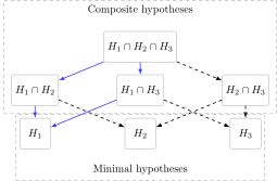
To reject the $H_{1}$ at an correct $\alpha$-level we should test all intersection hypotheses involving $H_{1}$ and check if there all are rejected at the $\alpha$-level. The adjusted $p$-values can here be obtained as the maximum $p$-value across all the composite hypothesis tests. Unfortunately, this only works for relatively few comparisons as the number of tests grows exponentially.

summary(closed_testing(gg0, test = test_wald, null=rep(.8, 3)))
#> Call: closed_testing(object = gg0, test = test_wald, null = rep(0.8, 
#>     3))
#>     Estimate     adj.p
#> a      1.403 1.060e-05
#> a.1    1.499 3.945e-07
#> a.2    1.359 3.958e-03
#> 1-way intersections:
#>   {a}                                      p = 0.0000
#>   {a.1}                                    p = 0.0000
#>   {a.2}                                    p = 0.0040
#> 
#> 2-way intersections:
#>   {a, a.1}                                 p = 0.0000
#>   {a, a.2}                                 p = 0.0000
#>   {a.1, a.2}                               p = 0.0000
#> 
#> 3-way intersections:
#>   {a, a.1, a.2}                            p = 0.0000

Averaging

Some parameters of interest are expressed as averages over functions of the observed data and estimated parameters of a model. The asymptotic distribution can in some of these cases also be derived from the influence function. Let $Z_{1},\ldots,Z_{n}$ be iid observations, $Z_{1}\sim P_{0}$ and let $X_{i}\subset Z_{i}$.

Lemma 3 Assume that $\widehat{\theta}$ is RAL estimator of $\theta\in\Omega\subset \mathbb{R}^{p}$$$\sqrt{n}(\widehat{\theta}-\theta) = \frac{1}{\sqrt{n}}\sum_{i=1}^{n}\phi(Z_{i}; P_{0}) + o_{P}(1).$$ Let $f:\mathcal{X}\times\Omega\to\mathbb{R}$ be continuous differentiable in $\theta$$$\sqrt{n}\{f(X; \widehat{\theta})-f(X; \theta)\} = \frac{1}{\sqrt{n}}\nabla_{\theta}f(X;\theta)\sum_{i=1}^{n}\phi(Z_{i}; P_{0}) + o_{P}(1).$$

Let $\Psi = P_{0}f(X;\theta)$ and $\widehat{\Psi} = P_{n} f(X;\widehat{\theta})$. $P_{0}$ and $P_{n}$ are here denoting the integrals wrt. $X$. Then the influence function for $\widehat{\Psi}$ is given by $$\begin{align*} IC(Z; P_{0}) = f(X;\theta)-\Psi + [P_{0}\nabla_{\theta}f(X;\theta)]\phi(Z). \end{align*}$$

Proof. It is easily verified that $$\begin{align*} \widehat{\Psi}-\Psi &= (P_{n}-P_{0})(f(X; \theta)-\Psi) + P[f(X;\widehat{\theta})-f(X;\theta)] \\ &\quad + (P_{n}-P_{0})[f(X;\widehat{\theta})-f(X;\theta)] \end{align*}$$

From Lemma 19.24 (Vaart 1998) it follows that for the last term $$\begin{align*} \sqrt{n}(P_{n}-P_{0})[f(X;\widehat{\theta})-f(X;\theta)] = o_{P}(1) \end{align*}$$ when $f$ for example is Lipschitz and more generally when $f(X;\theta)$ forms a $P_{0}$-Donsker class.

It therefore follows that $$\begin{align*} \sqrt{n}(\widehat{\Psi}-\Psi) &= \sqrt{n}P_{n}(f(X; \theta)-\Psi) + \frac{1}{\sqrt{n}}P\nabla_{\theta}f(X;\theta)\sum_{i=1}^{n}\phi(Z_{i}; P_{0}) + o_{P}(1) \\ &= \frac{1}{\sqrt{n}}\sum_{i=1}^{n}\{f(X;\theta)-\Psi\} + \frac{1}{\sqrt{n}}P\nabla_{\theta}f(X;\theta)\sum_{i=1}^{n}\phi(Z_{i}, P_{0}) + o_{P}(1) \end{align*}$$ Hence the IF for $\widehat{\Psi}$ becomes $$IC(Z; P_{0}) = f(X;\theta)-\Psi + [P_{0}\nabla_{\theta}f(X;\theta)]\phi(Z).$$

$\blacksquare$

Turning back to the example we can estimate the logistic regression model $\operatorname{logit}(E\{Y_1 | A,X_1,W\}) = \beta_0 + \beta_a A + \beta_{x_1} X_1 + \beta_w W$, and from this we want to estimate the target parameter $$\theta(P) = \mathbb{E}_{P}[E(Y\mid A=1, X_{1}, W)].$$ To do this we need first to estimate the model and then define a function that gives the predicted probability $\mathbb{P}(Y=1\mid A=1,X_{1},W)$ for any observed values of $X_1,W$ but with the treatment variable $A$ kept fixed at the value $1$

g <- glm(y1 ~ a + x1 + w, data=dw, family=binomial)
pr <- function(p, data, ...)
  with(data, expit(p[1] + p["a"] + p["x1"]*x1 + p["w"]*w))
pr(coef(g), dw) |> head()
#> [1] 0.7932 0.8968 0.3297 0.9425 0.7954 0.1948

The target parameter can now be estimated with the syntax

id <- foldr(NROW(dw), 100, list=FALSE)
ea <- estimate(g, pr, average=TRUE, id=id)
ea
#>     Estimate Std.Err   2.5%  97.5%    P-value
#> val   0.6628 0.02451 0.6148 0.7108 4.985e-161
IC(ea) |> head()
#>          val
#> 33   0.07714
#> 100  0.15616
#> 44   0.41135
#> 48  -0.13500
#> 16  -0.43901
#> 29  -0.05291

Average Treatment Effects

Let the observed data be $Z = (W,A,Y)$, where $W$ are covariates, $A$ a binary treatment variable, and $Y$ the outcome. In the following we are interested in estimating the target parameter $\psi_a(P) = E_P[Y(a)]$, where $Y(a)$ is the potential outcome we would have observed if treatment $a$ had been administered, possibly contrary to the actual treatment that was observed, i.e., $Y = Y(A)$. To assess the treatment effect we can then consider the average treatment effect (ATE) $$E_P[Y(1)]-E_P[Y(0)],$$ or some other contrast of interest $g(\psi_1(P), \psi_0(P))$. Under the following assumptions

1. Stable Unit Treatment Values Assumption (the treatment of a specific subject is not affecting the potential outcome of other subjects)
2. Positivity, $P(A=a\mid W)>\epsilon$ for some $\epsilon>0$ and baseline covariates $W$
3. No unmeasured confounders, $Y(a)\!\perp\!\!\!\!\perp\!A|W$

then the target parameter can be identified from the observed data distribution as $$E(E[Y|W,A=a]) = E(E[Y(a)|W]) = E[Y(a)]$$ or $$E[Y I(A=a)/P(A=a|W)] = E[Y(a)].$$

This suggests estimators based on outcome regression ($g$-computation) or inverse probability weighting. More generally, under the above assumption we can construct a one-step estimator from the Efficient Influence Function combining these two $$E\left[\frac{I(A=a)}{\Pi_a(W)}(Y-Q(W,A)) + Q(W,a)\right].$$ In practice, this requires plugin estimates of both the outcome model, $Q(W,A) := E(Y\mid A, W)$, and of the treatment propensity model $\Pi_a(W) := P(A=a\mid W)$. The corresponding estimator is consistent even if just one of the two nuisance models is correctly specified.

To illustrate this we manually construct the above estimating equations based on logistic regressions models for the two nuisance models

qmod <- glm(y1 ~ a * w, family = binomial, data = dw) # E(Y|W,A) := Q(W,A)
amod <- glm(a ~ w, family = binomial, data = dw) # P(A=1|W) = Pi_1(W)
q0 <- predict(qmod, transform(dw, a=0), type="response") # Q(W,0)
q1 <- predict(qmod, transform(dw, a=1), type="response") # Q(W,1)
p1 <- predict(amod, dw, type="response") # P(A=1|W)
e0 <- with(dw, (1-a) / (1-p1) * (y1 - q0) + q0)
e1 <- with(dw, a / p1 * (y1 - q1) + q1)
head(cbind(e0, e1))
#>         e0      e1
#> 1  0.65805  1.0545
#> 2  0.65453  1.0566
#> 3  0.33088  2.2411
#> 4  0.50712  1.2459
#> 5  0.48319 -0.7262
#> 6 -0.03954  0.3653

We can then easily construct estimates of the two expected potential outcomes and estimate their joint asymptotic distribution

est0 <- estimate(coef=mean(e0), IC=e0-mean(e0)) # E[Y(0)]
est1 <- estimate(coef=mean(e1), IC=e1-mean(e1)) # E[Y(1)]

potential_outcomes <- merge(est0, est1, paired=TRUE, labels=c("y(0)", "y(1)"))
potential_outcomes
#>      Estimate Std.Err   2.5%  97.5%    P-value
#> y(0)   0.4693 0.02355 0.4232 0.5155  2.187e-88
#> y(1)   0.6702 0.02454 0.6221 0.7183 3.657e-164
head(IC(potential_outcomes))
#>       y(0)    y(1)
#> 1  0.18872  0.3843
#> 2  0.18520  0.3865
#> 3 -0.13845  1.5709
#> 4  0.03779  0.5758
#> 5  0.01386 -1.3963
#> 6 -0.50886 -0.3049
vcov(potential_outcomes)
#>           y(0)      y(1)
#> y(0) 5.545e-04 2.385e-05
#> y(1) 2.385e-05 6.024e-04

Finally, we can obtain the Average Treatment Effect (ATE) (risk-difference) $$\begin{align*} E[Y(1)] - E[Y(0)] \end{align*}$$

estimate(potential_outcomes, cbind(-1, 1), labels="ate")
#>     Estimate Std.Err   2.5%  97.5%   P-value
#> ate   0.2008  0.0333 0.1356 0.2661 1.637e-09

Alternatively, we could get the estimate of the treatment effect on the log-odds scale:

est <- with(potential_outcomes, logit(`y(1)`)-logit(`y(0)`))
est
#>      Estimate Std.Err   2.5% 97.5%   P-value
#> y(1)   0.8317  0.1428 0.5518 1.112 5.768e-09
transform(est, labels="OR") |>
  summary(transform = exp)
#> Call: estimate.default(x = `_data`, labels = "OR")
#> ────────────────────────────────────────────────────────────
#>    Estimate Std.Err  2.5% 97.5%   P-value
#> OR    2.297         1.736 3.039 5.768e-09
#> ────────────────────────────────────────────────────────────
#> Null Hypothesis: 
#>   [OR] = 0 
#>  
#> chisq = 33.91, df = 1, p-value = 5.768e-09
#logor <- function(p) logit(p[2]) - logit(p[1])
#transform(potential_outcomes, logor, labels="logOR")
#transform(potential_outcomes, logor, labels="OR") |> summary(transform = exp)

We refer to the targeted package (Holst et al. 2026) for a general implementation where the nuisance models can be based on machine learning models using cross-fitting. The above estimation can be obtained with the targeted::cate function in the following way

amod <- targeted::learner_glm(a ~ w, family=binomial)
qmod <- targeted::learner_glm(y1 ~ a * w, family=binomial)
est <- targeted::cate(qmod, amod, data=dw, second.order = FALSE)
#>             Estimate Std.Err    2.5%  97.5%   P-value
#> E[y1(1)]      0.7050 0.03721 0.63207 0.7779 4.934e-80
#> E[y1(0)]      0.5359 0.03535 0.46666 0.6052 6.290e-52
#> ───────────
#> (Intercept)   0.1691 0.04996 0.07115 0.2670 7.138e-04

SessionInfo

sessionInfo()
#> R version 4.6.1 (2026-06-24)
#> Platform: x86_64-pc-linux-gnu
#> Running under: Ubuntu 24.04.4 LTS
#> 
#> Matrix products: default
#> BLAS:   /usr/lib/x86_64-linux-gnu/openblas-pthread/libblas.so.3 
#> LAPACK: /usr/lib/x86_64-linux-gnu/openblas-pthread/libopenblasp-r0.3.26.so;  LAPACK version 3.12.0
#> 
#> locale:
#>  [1] LC_CTYPE=C.UTF-8       LC_NUMERIC=C           LC_TIME=C.UTF-8       
#>  [4] LC_COLLATE=C.UTF-8     LC_MONETARY=C.UTF-8    LC_MESSAGES=C.UTF-8   
#>  [7] LC_PAPER=C.UTF-8       LC_NAME=C              LC_ADDRESS=C          
#> [10] LC_TELEPHONE=C         LC_MEASUREMENT=C.UTF-8 LC_IDENTIFICATION=C   
#> 
#> time zone: UTC
#> tzcode source: system (glibc)
#> 
#> attached base packages:
#> [1] stats     graphics  grDevices utils     datasets  methods   base     
#> 
#> other attached packages:
#> [1] survival_3.8-6 lava_1.9.3    
#> 
#> loaded via a namespace (and not attached):
#>  [1] Matrix_1.7-5           future.apply_1.20.2    jsonlite_2.0.0        
#>  [4] dplyr_1.2.1            compiler_4.6.1         tidyselect_1.2.1      
#>  [7] Rcpp_1.1.2             parallel_4.6.1         tidyr_1.3.2           
#> [10] globals_0.19.1         splines_4.6.1          yaml_2.3.12           
#> [13] fastmap_1.2.0          lattice_0.22-9         R6_2.6.1              
#> [16] generics_0.1.4         knitr_1.51             backports_1.5.1       
#> [19] MASS_7.3-65            tibble_3.3.1           future_1.75.0         
#> [22] pillar_1.11.1          rlang_1.3.0            broom_1.0.13          
#> [25] xfun_0.60              otel_0.2.0             cli_3.6.6             
#> [28] magrittr_2.0.5         digest_0.6.39          grid_4.6.1            
#> [31] mvtnorm_1.4-2          geepack_1.3.13         lifecycle_1.0.5       
#> [34] RcppArmadillo_15.4.2-1 timereg_2.0.7          vctrs_0.7.3           
#> [37] evaluate_1.0.5         glue_1.8.1             numDeriv_2016.8-1.1   
#> [40] listenv_1.0.0          codetools_0.2-20       parallelly_1.48.0     
#> [43] purrr_1.2.2            rmarkdown_2.31         pkgconfig_2.0.3       
#> [46] tools_4.6.1            htmltools_0.5.9        mets_1.3.12

Bibliography

Bickel, Peter J., Chris A. J. Klaassen, Ya’Acov Ritov, and Jon A. Wellner. 1998. Efficient and Adaptive Estimation for Semiparametric Models. Springer.

Halekoh, Ulrich, Søren Højsgaard, and Jun Yan. 2006. “The R Package Geepack for Generalized Estimating Equations.” Journal of Statistical Software 15/2: 1–11. https://doi.org/10.18637/jss.v015.i02.

Hines, Oliver, Oliver Dukes, Karla Diaz-Ordaz, and Stijn Vansteelandt. 2022. “Demystifying Statistical Learning Based on Efficient Influence Functions.” The American Statistician, February, 1–13. https://doi.org/10.1080/00031305.2021.2021984.

Holst, K. K., and E. Budtz-Jørgensen. 2013. “Linear Latent Variable Models: The Lava-Package.” Computational Statistics 28 (4): 1385–452. https://doi.org/10.1007/s00180-012-0344-y.

Holst, Klaus K., Benedikt Sommer, and Andreas Nordland. 2026. Targeted: Targeted Inference. https://kkholst.github.io/targeted/.

Laan, Mark J. van der, and Sherri Rose. 2011. Targeted Learning. Causal Inference for Observational and Experimental Data. Springer. https://doi.org/10.1007/978-1-4419-9782-1.

Lehmann, E. L., and Joseph P. Romano. 2023. Testing Statistical Hypotheses. Fourth. Springer Texts in Statistics. Springer. https://doi.org/10.1007/978-3-030-70578-7.

Marcus, Ruth, Eric Pertiz, and K. R. Gabriel. 1976. “On Closed Testing Procedures with Special Reference to Ordered Analysis of Variance.” Biometrika 63 (3): 655–60. https://doi.org/10.1093/biomet/63.3.655.

Pipper, Christian B., Christian Ritz, and Hans Bisgaard. 2012. “A Versatile Method for Confirmatory Evaluation of the Effects of a Covariate in Multiple Models.” Journal of the Royal Statistical Society C, Appl. Statist. 61 (2): 315–26. https://doi.org/10.1111/j.1467-9876.2011.01005.x.

Therneau, T., and P. Grambsch. 2000. Modeling Survival Data: Extending the Cox Model. Springer-Verlag, New York. https://doi.org/10.1007/978-1-4757-3294-8.

Tsiatis, A. 2006. Semiparametric Theory and Missing Data. Springer Series in Statistics. Springer New York. https://doi.org/10.1007/0-387-37345-4.

Vaart, A. W. van der. 1998. Asymptotic Statistics. In Cambridge University Press, Cambridge. https://doi.org/10.1017/CBO9780511802256.

Zeileis, Achim, Susanne Köll, and Nathaniel Graham. 2020. “Various Versatile Variances: An Object-Oriented Implementation of Clustered Covariances in R.” Journal of Statistical Software 95 (1): 1–36. https://doi.org/10.18637/jss.v095.i01.

Zeng, Donglin, and D. Y. Lin. 2008. “Efficient Resampling Methods for Nonsmooth Estimating Functions.” Biostatistics 9 (2): 355–63. https://doi.org/10.1093/biostatistics/kxm034.