twSigmaLogitnorm

Estimating coefficients of logitnormal distribution from mode and given mu

twSigmaLogitnorm(mle, mu = 0)

Arguments

mle

numeric vector: the mode of the density function

mu

for mu = 0 the distribution will be the flattest case (maybe bimodal)

Details

For a mostly flat unimodal distribution use twCoefLogitnormMLE(mle,0)

Value

numeric matrix with columns c("mu","sigma") rows correspond to rows in mle and mu

Author

Thomas Wutzler

See also

logitnorm

Examples

mle <- 0.8
(theta <- twSigmaLogitnorm(mle))
#>      mu   sigma
#> [1,]  0 1.52003
#
x <- seq(0,1,length.out = 41)[-c(1,41)]  # plotting grid
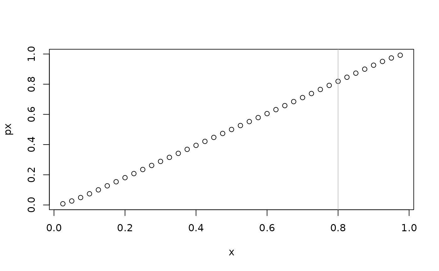
px <- plogitnorm(x,mu = theta[1],sigma = theta[2])  #percentiles function
plot(px~x); abline(v = c(mle),col = "gray")

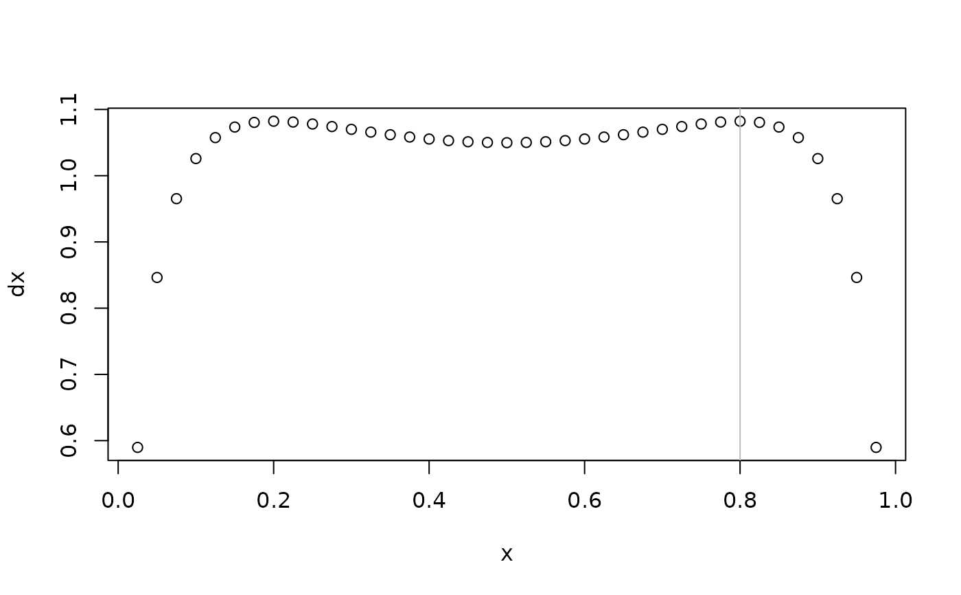
dx <- dlogitnorm(x,mu = theta[1],sigma = theta[2])  #density function
plot(dx~x); abline(v = c(mle),col = "gray")

# vectorized
(theta <- twSigmaLogitnorm(mle = seq(0.401,0.8,by = 0.1)))
#>      mu    sigma
#> [1,]  0 1.423646
#> [2,]  0 1.414215
#> [3,]  0 1.424040
#> [4,]  0 1.455872