Censored Box-Cox Gaussian family
bcg.RdFamily for use with gam or bam, implementing regression for censored
data that can be modelled as Gaussian after Box-Cox transformation. If \(y>0\) is the response and
$$z= \left \{ \begin{array}{ll} (y^\lambda-1)/\lambda & \lambda \ne 0 \\ \log(y) & \lambda =0
\end{array} \right . $$
with mean \(\mu\) and standard deviation \(w^{-1/2}\exp(\theta)\),
then \(w^{1/2}(z-\mu)\exp(-\theta)\) follows an \(N(0,1)\) distribution. That is
$$z \sim N(\mu,e^{2\theta}w^{-1}).$$ \(\theta\) is a single scalar for all observations, and similarly Box-Cox parameter \(\lambda\) is a single scalar. Observations may be left, interval or right censored or uncensored.
Note that the regression model here specifies the mean of the Box-Cox transformed response, not the mean of the response itself: this is rather different to the usual GLM approach.
bcg(theta=NULL,link="identity")Arguments
- theta
a 2-vector containing the Box-Cox parameter \(\lambda\) and the log standard deviation parameter \(\theta\). If supplied and positive then taken as a fixed value of \(\lambda\) and \(\exp(\theta)\). If supplied and second element negative taken as initial value and negative of initial value respectively.
- link
The link function:
"identity","log"or"sqrt".
Value
An object of class extended.family.
Details
If the family is used with a vector response, then it is assumed that there is no censoring. If there is censoring then the response should be supplied as a two column matrix. The first column is always numeric. Entries in the second column are as follows.
If an entry is identical to the corresponding first column entry, then it is an uncensored observation.
If an entry is numeric and different to the first column entry then there is interval censoring. The first column entry is the lower interval limit and the second column entry is the upper interval limit. \(y\) is only known to be between these limits.
If the second column entry is
0then the observation is left censored at the value of the entry in the first column. It is only known that \(y\) is less than or equal to the first column value.If the second column entry is
Infthen the observation is right censored at the value of the entry in the first column. It is only known that \(y\) is greater than or equal to the first column value.
Any mixture of censored and uncensored data is allowed, but be aware that data consisting only of right and/or left censored data contain very little information.
References
Wood, S.N., N. Pya and B. Saefken (2016), Smoothing parameter and model selection for general smooth models. Journal of the American Statistical Association 111, 1548-1575 doi:10.1080/01621459.2016.1180986
Examples
library(mgcv)
set.seed(3) ## Simulate some gamma data?
dat <- gamSim(1,n=400,dist="normal",scale=1)
#> Gu & Wahba 4 term additive model
dat$f <- dat$f/4 ## true linear predictor
Ey <- exp(dat$f);scale <- .5 ## mean and GLM scale parameter
dat$y <- rgamma(Ey*0,shape=1/scale,scale=Ey*scale)
## Just Box-Cox no censoring...
b <- gam(y~s(x0)+s(x1)+s(x2)+s(x3),family=bcg,data=dat)
summary(b)
#>
#> Family: bcg(0.079,0.928)
#> Link function: identity
#>
#> Formula:
#> y ~ s(x0) + s(x1) + s(x2) + s(x3)
#>
#> Parametric coefficients:
#> Estimate Std. Error z value Pr(>|z|)
#> (Intercept) 1.9160 0.0464 41.29 <2e-16 ***
#> ---
#> Signif. codes: 0 ‘***’ 0.001 ‘**’ 0.01 ‘*’ 0.05 ‘.’ 0.1 ‘ ’ 1
#>
#> Approximate significance of smooth terms:
#> edf Ref.df Chi.sq p-value
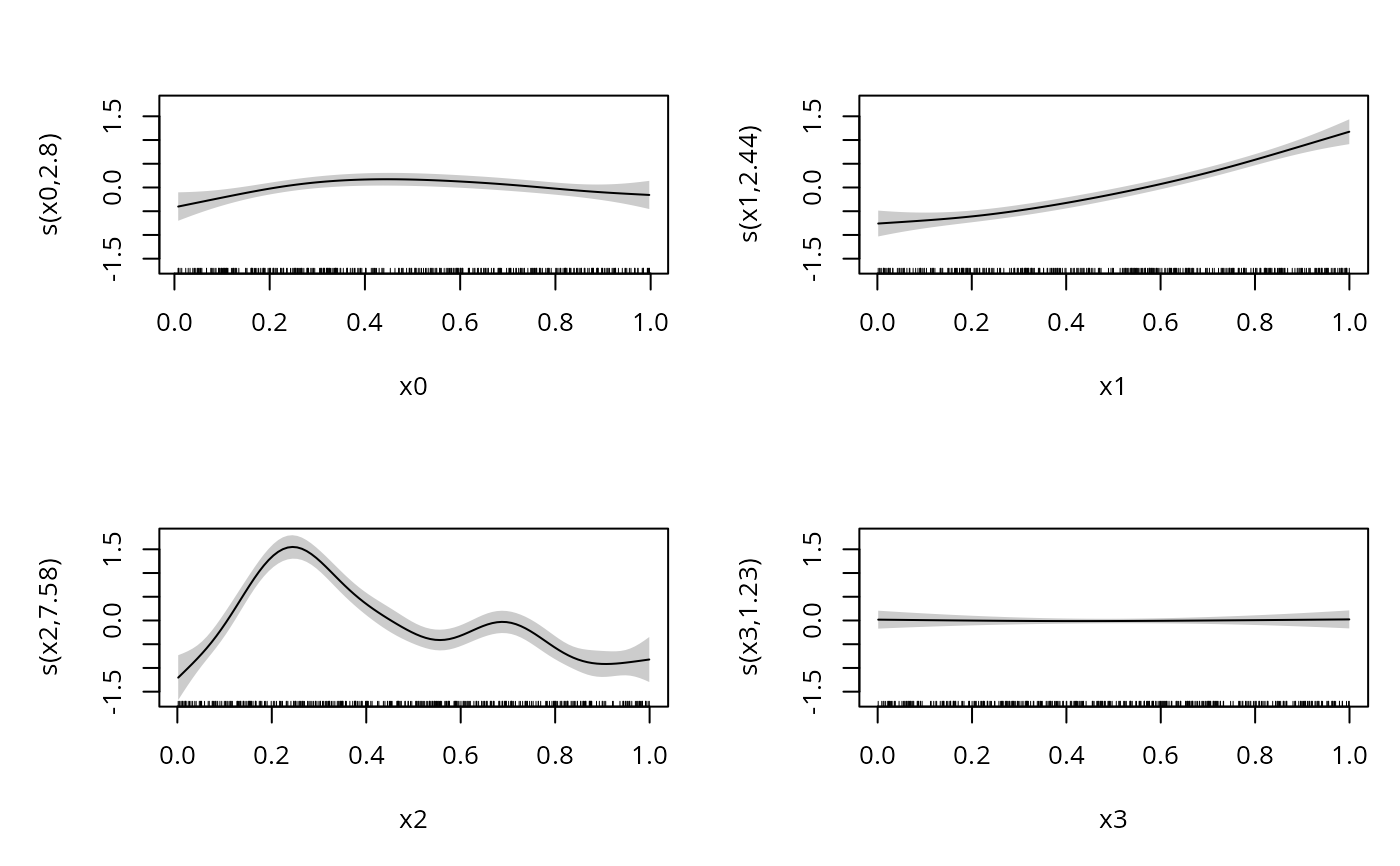
#> s(x0) 2.798 3.483 10.88 0.0187 *
#> s(x1) 2.441 3.038 152.84 <2e-16 ***
#> s(x2) 7.585 8.483 265.46 <2e-16 ***
#> s(x3) 1.229 1.422 0.08 0.9132
#> ---
#> Signif. codes: 0 ‘***’ 0.001 ‘**’ 0.01 ‘*’ 0.05 ‘.’ 0.1 ‘ ’ 1
#>
#> R-sq.(adj) = 0.0527 Deviance explained = 52.1%
#> -REML = 1198.6 Scale est. = 1 n = 400
plot(b,pages=1,scheme=1)
 ## try various censoring...
yb <- cbind(dat$y,dat$y)
ind <- 1:100
yb[ind,2] <- yb[ind,1] + runif(100)*3
yb[51:100,2] <- 0 ## left censored
yb[101:140,2] <- Inf ## right censored
b <- gam(yb~s(x0)+s(x1)+s(x2)+s(x3),family=bcg,data=dat)
summary(b)
#>
#> Family: bcg(0.05,0.948)
#> Link function: identity
#>
#> Formula:
#> yb ~ s(x0) + s(x1) + s(x2) + s(x3)
#>
#> Parametric coefficients:
#> Estimate Std. Error z value Pr(>|z|)
#> (Intercept) 1.84207 0.04977 37.01 <2e-16 ***
#> ---
#> Signif. codes: 0 ‘***’ 0.001 ‘**’ 0.01 ‘*’ 0.05 ‘.’ 0.1 ‘ ’ 1
#>
#> Approximate significance of smooth terms:
#> edf Ref.df Chi.sq p-value
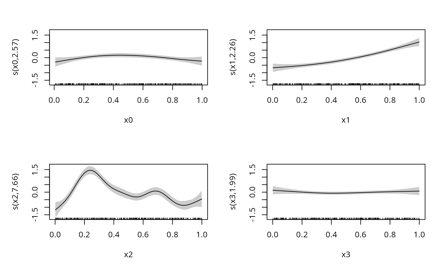
#> s(x0) 2.568 3.199 8.111 0.0506 .
#> s(x1) 2.256 2.808 103.527 <2e-16 ***
#> s(x2) 7.661 8.533 192.256 <2e-16 ***
#> s(x3) 1.990 2.480 1.032 0.5643
#> ---
#> Signif. codes: 0 ‘***’ 0.001 ‘**’ 0.01 ‘*’ 0.05 ‘.’ 0.1 ‘ ’ 1
#>
#> R-sq.(adj) = 0.0429 Deviance explained = 42%
#> -REML = 1008.3 Scale est. = 1 n = 400
plot(b,pages=1,scheme=1)
## try various censoring...
yb <- cbind(dat$y,dat$y)
ind <- 1:100
yb[ind,2] <- yb[ind,1] + runif(100)*3
yb[51:100,2] <- 0 ## left censored
yb[101:140,2] <- Inf ## right censored
b <- gam(yb~s(x0)+s(x1)+s(x2)+s(x3),family=bcg,data=dat)
summary(b)
#>
#> Family: bcg(0.05,0.948)
#> Link function: identity
#>
#> Formula:
#> yb ~ s(x0) + s(x1) + s(x2) + s(x3)
#>
#> Parametric coefficients:
#> Estimate Std. Error z value Pr(>|z|)
#> (Intercept) 1.84207 0.04977 37.01 <2e-16 ***
#> ---
#> Signif. codes: 0 ‘***’ 0.001 ‘**’ 0.01 ‘*’ 0.05 ‘.’ 0.1 ‘ ’ 1
#>
#> Approximate significance of smooth terms:
#> edf Ref.df Chi.sq p-value
#> s(x0) 2.568 3.199 8.111 0.0506 .
#> s(x1) 2.256 2.808 103.527 <2e-16 ***
#> s(x2) 7.661 8.533 192.256 <2e-16 ***
#> s(x3) 1.990 2.480 1.032 0.5643
#> ---
#> Signif. codes: 0 ‘***’ 0.001 ‘**’ 0.01 ‘*’ 0.05 ‘.’ 0.1 ‘ ’ 1
#>
#> R-sq.(adj) = 0.0429 Deviance explained = 42%
#> -REML = 1008.3 Scale est. = 1 n = 400
plot(b,pages=1,scheme=1)