Generate inverse Gaussian random deviates

Generates inverse Gaussian random deviates.

rig(n,mean,scale)

Arguments

n

the number of deviates required. If this has length > 1 then the length is taken as the number of deviates required.

mean

vector of mean values.

scale

vector of scale parameter values (lambda, see below)

Value

A vector of inverse Gaussian random deviates.

Details

If x if the returned vector, then E(x) = mean while var(x) = scale*mean^3. For density and distribution functions see the statmod package. The algorithm used is Algorithm 5.7 of Gentle (2003), based on Michael et al. (1976). Note that scale here is the scale parameter in the GLM sense, which is the reciprocal of the usual `lambda' parameter.

References

Gentle, J.E. (2003) Random Number Generation and Monte Carlo Methods (2nd ed.) Springer.

Michael, J.R., W.R. Schucany & R.W. Hass (1976) Generating random variates using transformations with multiple roots. The American Statistician 30, 88-90.

Author

Simon N. Wood simon.wood@r-project.org

Examples

require(mgcv)
set.seed(7)
## An inverse.gaussian GAM example, by modify `gamSim' output... 
dat <- gamSim(1,n=400,dist="normal",scale=1)
#> Gu & Wahba 4 term additive model
dat$f <- dat$f/4 ## true linear predictor 
Ey <- exp(dat$f);scale <- .5 ## mean and GLM scale parameter
## simulate inverse Gaussian response...
dat$y <- rig(Ey,mean=Ey,scale=.2)
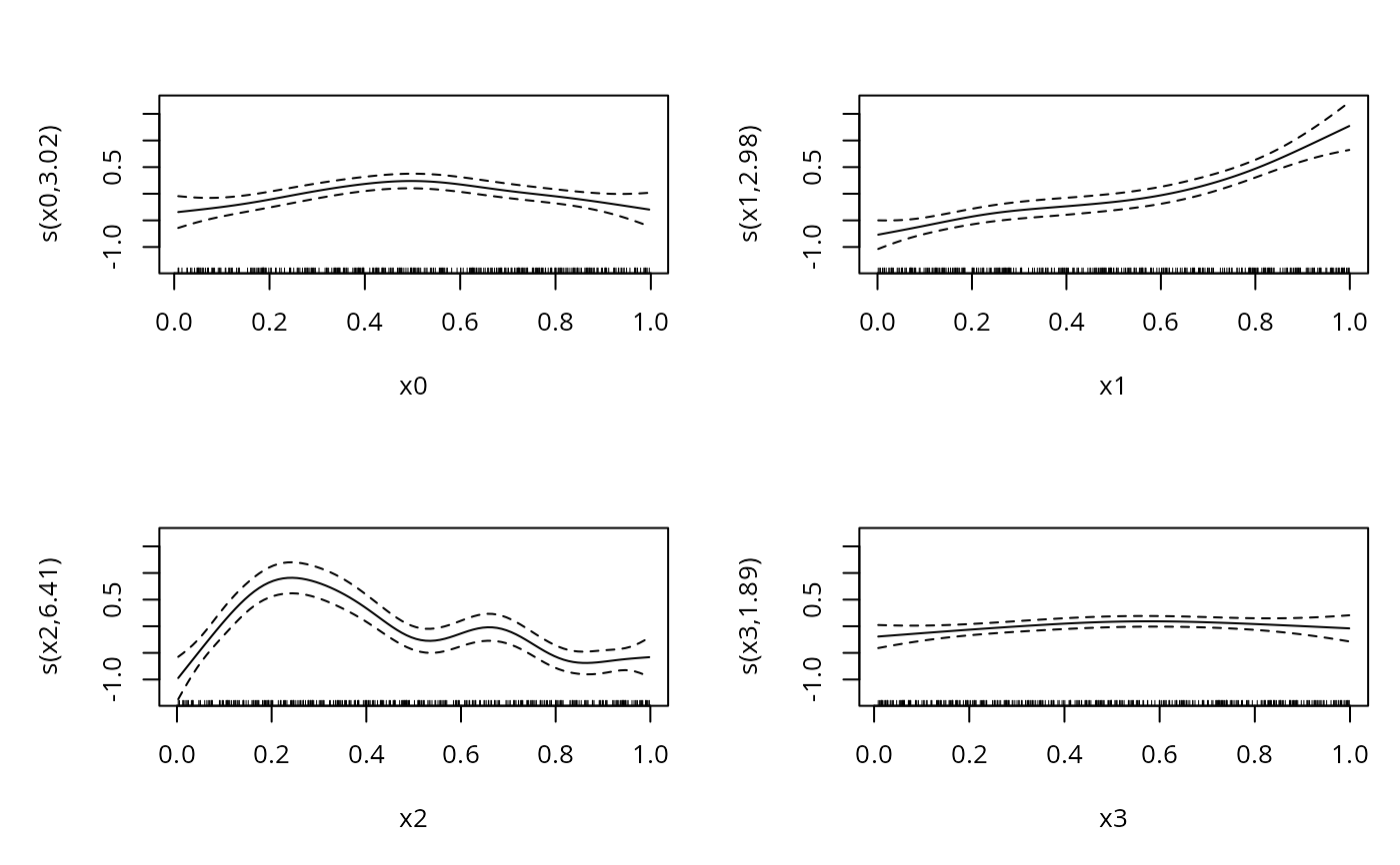
big <- gam(y~ s(x0)+ s(x1)+s(x2)+s(x3),family=inverse.gaussian(link=log),
          data=dat,method="REML")
plot(big,pages=1)

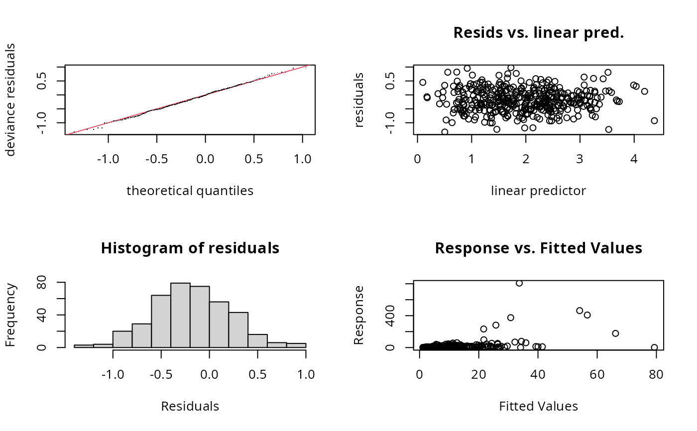
gam.check(big)

#> 
#> Method: REML   Optimizer: outer newton
#> full convergence after 8 iterations.
#> Gradient range [-0.0003256568,4.561143e-06]
#> (score 1154.207 & scale 0.1808111).
#> Hessian positive definite, eigenvalue range [0.2487389,197.5501].
#> Model rank =  37 / 37 
#> 
#> Basis dimension (k) checking results. Low p-value (k-index<1) may
#> indicate that k is too low, especially if edf is close to k'.
#> 
#>         k'  edf k-index p-value  
#> s(x0) 9.00 3.02    0.76   0.075 .
#> s(x1) 9.00 2.98    0.89   0.935  
#> s(x2) 9.00 6.41    0.85   0.665  
#> s(x3) 9.00 1.89    0.89   0.950  
#> ---
#> Signif. codes:  0 ‘***’ 0.001 ‘**’ 0.01 ‘*’ 0.05 ‘.’ 0.1 ‘ ’ 1
summary(big)
#> 
#> Family: inverse.gaussian 
#> Link function: log 
#> 
#> Formula:
#> y ~ s(x0) + s(x1) + s(x2) + s(x3)
#> 
#> Parametric coefficients:
#>             Estimate Std. Error t value Pr(>|t|)    
#> (Intercept)  1.93014    0.06261   30.83   <2e-16 ***
#> ---
#> Signif. codes:  0 ‘***’ 0.001 ‘**’ 0.01 ‘*’ 0.05 ‘.’ 0.1 ‘ ’ 1
#> 
#> Approximate significance of smooth terms:
#>         edf Ref.df      F p-value    
#> s(x0) 3.020  3.744  3.894 0.00556 ** 
#> s(x1) 2.985  3.712 20.371 < 2e-16 ***
#> s(x2) 6.412  7.524 12.139 < 2e-16 ***
#> s(x3) 1.887  2.343  1.637 0.16824    
#> ---
#> Signif. codes:  0 ‘***’ 0.001 ‘**’ 0.01 ‘*’ 0.05 ‘.’ 0.1 ‘ ’ 1
#> 
#> R-sq.(adj) =  0.0874   Deviance explained = 38.6%
#> -REML = 1154.2  Scale est. = 0.18081   n = 400