Zero inflated (hurdle) Poisson location-scale model family
ziplss.RdThe ziplss family implements a zero inflated (hurdle) Poisson model in which one linear predictor
controls the probability of presence and the other controls the mean given presence.
Useable only with gam, the linear predictors are specified via a list of formulae.
Should be used with care: simply having a large number of zeroes is not an indication of zero inflation.
Requires integer count data.
ziplss(link=list("identity","identity"))
zipll(y,g,eta,deriv=0)
Arguments
Value
For ziplss An object inheriting from class general.family.
Details
ziplss is used with gam to fit 2 stage zero inflated Poisson models. gam is called with
a list containing 2 formulae, the first specifies the response on the left hand side and the structure of the linear predictor for the Poisson parameter on the right hand side. The second is one sided, specifying the linear predictor for the probability of presence on the right hand side.
The fitted values for this family will be a two column matrix. The first column is the log of the Poisson parameter,
and the second column is the complementary log log of probability of presence..
Predictions using predict.gam will also produce 2 column matrices for type
"link" and "response".
The null deviance computed for this model assumes that a single probability of presence and a single Poisson parameter are estimated.
For data with large areas of covariate space over which the response is zero it may be advisable to use low order penalties to
avoid problems. For 1D smooths uses e.g. s(x,m=1) and for isotropic smooths use Duchon.splines in place of thin plaste terms with order 1 penalties, e.g s(x,z,m=c(1,.5)) — such smooths penalize towards constants, thereby avoiding extreme estimates when the data are uninformative.
zipll is a function used by ziplss, exported only to allow external use of the ziplss family. It is not usually called directly.
References
Wood, S.N., N. Pya and B. Saefken (2016), Smoothing parameter and model selection for general smooth models. Journal of the American Statistical Association 111, 1548-1575 doi:10.1080/01621459.2016.1180986
WARNINGS
Zero inflated models are often over-used. Having many zeroes in the data does not in itself imply zero inflation. Having too many zeroes *given the model mean* may imply zero inflation.
Examples
library(mgcv)
## simulate some data...
f0 <- function(x) 2 * sin(pi * x); f1 <- function(x) exp(2 * x)
f2 <- function(x) 0.2 * x^11 * (10 * (1 - x))^6 + 10 *
(10 * x)^3 * (1 - x)^10
n <- 500;set.seed(5)
x0 <- runif(n); x1 <- runif(n)
x2 <- runif(n); x3 <- runif(n)
## Simulate probability of potential presence...
eta1 <- f0(x0) + f1(x1) - 3
p <- binomial()$linkinv(eta1)
y <- as.numeric(runif(n)<p) ## 1 for presence, 0 for absence
## Simulate y given potentially present (not exactly model fitted!)...
ind <- y>0
eta2 <- f2(x2[ind])/3
y[ind] <- rpois(exp(eta2),exp(eta2))
## Fit ZIP model...
b <- gam(list(y~s(x2)+s(x3),~s(x0)+s(x1)),family=ziplss())
b$outer.info ## check convergence
#> $conv
#> [1] "full convergence"
#>
#> $iter
#> [1] 8
#>
#> $grad
#> [,1]
#> [1,] -1.161134e-08
#> [2,] -8.222732e-08
#> [3,] -7.874008e-05
#> [4,] -2.267803e-04
#>
#> $hess
#> [,1] [,2] [,3] [,4]
#> [1,] 3.444648809 0.004440335 0.000000e+00 0.000000e+00
#> [2,] 0.004440335 0.008865299 0.000000e+00 0.000000e+00
#> [3,] 0.000000000 0.000000000 1.363297e+00 8.321279e-05
#> [4,] 0.000000000 0.000000000 8.321279e-05 2.281058e-04
#>
#> $score.hist
#> [1] 882.3799 879.3079 879.1115 879.0838 879.0754 879.0725 879.0715 879.0711
#>
summary(b)
#>
#> Family: ziplss
#> Link function: identity identity
#>
#> Formula:
#> y ~ s(x2) + s(x3)
#> <environment: 0x5efde989f8d0>
#> ~s(x0) + s(x1)
#> <environment: 0x5efde989f8d0>
#>
#> Parametric coefficients:
#> Estimate Std. Error z value Pr(>|z|)
#> (Intercept) 1.14488 0.04888 23.420 <2e-16 ***
#> (Intercept).1 -0.05605 0.06467 -0.867 0.386
#> ---
#> Signif. codes: 0 ‘***’ 0.001 ‘**’ 0.01 ‘*’ 0.05 ‘.’ 0.1 ‘ ’ 1
#>
#> Approximate significance of smooth terms:
#> edf Ref.df Chi.sq p-value
#> s(x2) 8.025 8.714 1071.347 < 2e-16 ***
#> s(x3) 1.148 1.281 0.208 0.864
#> s.1(x0) 3.869 4.787 31.415 9.14e-06 ***
#> s.1(x1) 1.003 1.005 70.549 < 2e-16 ***
#> ---
#> Signif. codes: 0 ‘***’ 0.001 ‘**’ 0.01 ‘*’ 0.05 ‘.’ 0.1 ‘ ’ 1
#>
#> Deviance explained = 61.6%
#> -REML = 879.07 Scale est. = 1 n = 500
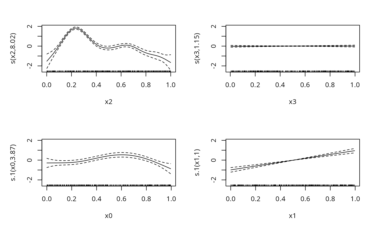
plot(b,pages=1)