Prediction from fitted GAM model
predict.gam.RdTakes a fitted gam object produced by gam()
and produces predictions given a new set of values for the model covariates
or the original values used for the model fit. Predictions can be accompanied
by standard errors, based on the posterior distribution of the model
coefficients. The routine can optionally return the matrix by which the model
coefficients must be pre-multiplied in order to yield the values of the linear predictor at
the supplied covariate values: this is useful for obtaining credible regions
for quantities derived from the model (e.g. derivatives of smooths), and for lookup table prediction outside
R (see example code below).
# S3 method for class 'gam'
predict(object,newdata,type="link",se.fit=FALSE,terms=NULL,
        exclude=NULL,block.size=NULL,newdata.guaranteed=FALSE,
        na.action=na.pass,unconditional=FALSE,iterms.type=NULL,...)
Arguments
- object
a fitted
gamobject as produced bygam().- newdata
A data frame or list containing the values of the model covariates at which predictions are required. If this is not provided then predictions corresponding to the original data are returned. If
newdatais provided then it should contain all the variables needed for prediction: a warning is generated if not. See details for use withlink{linear.functional.terms}.- type
When this has the value
"link"(default) the linear predictor (possibly with associated standard errors) is returned. Whentype="terms"each component of the linear predictor is returned seperately (possibly with standard errors): this includes parametric model components, followed by each smooth component, but excludes any offset and any intercept.type="iterms"is the same, except that any standard errors returned for smooth components will include the uncertainty about the intercept/overall mean. Whentype="response"predictions on the scale of the response are returned (possibly with approximate standard errors). Whentype="lpmatrix"then a matrix is returned which yields the values of the linear predictor (minus any offset) when postmultiplied by the parameter vector (in this casese.fitis ignored). The latter option is most useful for getting variance estimates for quantities derived from the model: for example integrated quantities, or derivatives of smooths. A linear predictor matrix can also be used to implement approximate prediction outsideR(see example code, below).- se.fit
when this is TRUE (not default) standard error estimates are returned for each prediction. If set to a number between 0 and 1 then this is taken as the confidence level for intervals that are returned instead.
- terms
if
type=="terms"ortype="iterms"then only results for the terms (smooth or parametric) named in this array will be returned. Otherwise any terms not named in this array will be set to zero. IfNULLthen all terms are included.- exclude
if
type=="terms"ortype="iterms"then terms (smooth or parametric) named in this array will not be returned. Otherwise any terms named in this array will be set to zero. IfNULLthen no terms are excluded. Note that this is the term names as it appears in the model summary, see example. You can avoid providing the covariates for excluded smooth terms by settingnewdata.guaranteed=TRUE, which will avoid all checks onnewdata(covariates for parametric terms can not be skipped).- block.size
maximum number of predictions to process per call to underlying code: larger is quicker, but more memory intensive. Set to < 1 to use total number of predictions as this. If
NULLthen block size is 1000 if new data supplied, and the number of rows in the model frame otherwise.- newdata.guaranteed
Set to
TRUEto turn off all checking ofnewdataexcept for sanity of factor levels: this can speed things up for large prediction tasks, butnewdatamust be complete, with noNAvalues for predictors required in the model.- na.action
what to do about
NAvalues innewdata. With the defaultna.pass, any row ofnewdatacontainingNAvalues for required predictors, gives rise toNApredictions (even if the term concerned has noNApredictors).na.excludeorna.omitresult in the dropping ofnewdatarows, if they contain anyNAvalues for required predictors. Ifnewdatais missing thenNAhandling is determined fromobject$na.action.- unconditional
if
TRUEthen the smoothing parameter uncertainty corrected covariance matrix is used, when available, otherwise the covariance matrix conditional on the estimated smoothing parameters is used.- iterms.type
if
type="iterms"then standard errors can either include the uncertainty in the overall mean (default, withfixed and random effects included) or the uncertainty in the mean of the non-smooth fixed effects only (iterms.type=2).- ...
other arguments.
Value
If type=="lpmatrix" then a matrix is returned which will
give a vector of linear predictor values (minus any offest) at the supplied covariate
values, when applied to the model coefficient vector.
Otherwise, if se.fit is TRUE then a 2 item list is returned with items (both arrays) fit
and se.fit containing predictions and associated standard error estimates, otherwise an
array of predictions is returned. The dimensions of the returned arrays depends on whether
type is "terms" or not: if it is then the array is 2 dimensional with each
term in the linear predictor separate, otherwise the array is 1 dimensional and contains the
linear predictor/predicted values (or corresponding s.e.s). The linear predictor returned termwise will
not include the offset or the intercept. If se.fit is a number between 0 and 1 then in place of se.fit two arrays are returned ll and ul giving the confidence interval limits.
newdata can be a data frame, list or model.frame: if it's a model frame
then all variables must be supplied.
Details
The standard errors produced by predict.gam are based on the
Bayesian posterior covariance matrix of the parameters Vp in the fitted
gam object.
When predicting from models with linear.functional.terms then there are two possibilities. If the summation convention is to be used in prediction, as it was in fitting, then newdata should be a list, with named matrix arguments corresponding to any variables that were matrices in fitting. Alternatively one might choose to simply evaluate the constitutent smooths at particular values in which case arguments that were matrices can be replaced by vectors (and newdata can be a dataframe). See linear.functional.terms for example code.
To facilitate plotting with termplot, if object possesses
an attribute "para.only" and type=="terms" then only parametric
terms of order 1 are returned (i.e. those that termplot can handle).
Note that, in common with other prediction functions, any offset supplied to
gam as an argument is always ignored when predicting, unlike
offsets specified in the gam model formula.
See the examples for how to use the lpmatrix for obtaining credible
regions for quantities derived from the model.
References
Chambers and Hastie (1993) Statistical Models in S. Chapman & Hall.
Marra, G and S.N. Wood (2012) Coverage Properties of Confidence Intervals for Generalized Additive Model Components. Scandinavian Journal of Statistics, 39(1), 53-74. doi:10.1111/j.1467-9469.2011.00760.x
Wood S.N. (2017, 2nd ed) Generalized Additive Models: An Introduction with R. Chapman and Hall/CRC Press. doi:10.1201/9781315370279
WARNING
Predictions are likely to be incorrect if data dependent transformations of the covariates are used within calls to smooths. See examples.
Note that the behaviour of this function is not identical to
predict.gam() in Splus.
type=="terms" does not exactly match what predict.lm does for
parametric model components.
Examples
library(mgcv)
n <- 200
sig <- 2
dat <- gamSim(1,n=n,scale=sig)
#> Gu & Wahba 4 term additive model
b <- gam(y~s(x0)+s(I(x1^2))+s(x2)+offset(x3),data=dat)
newd <- data.frame(x0=(0:30)/30,x1=(0:30)/30,x2=(0:30)/30,x3=(0:30)/30)
pred <- predict.gam(b,newd)
pred0 <- predict(b,newd,exclude="s(x0)") ## prediction excluding a term
## ...and the same, but without needing to provide x0 prediction data...
newd1 <- newd;newd1$x0 <- NULL ## remove x0 from `newd1'
pred1 <- predict(b,newd1,exclude="s(x0)",newdata.guaranteed=TRUE)
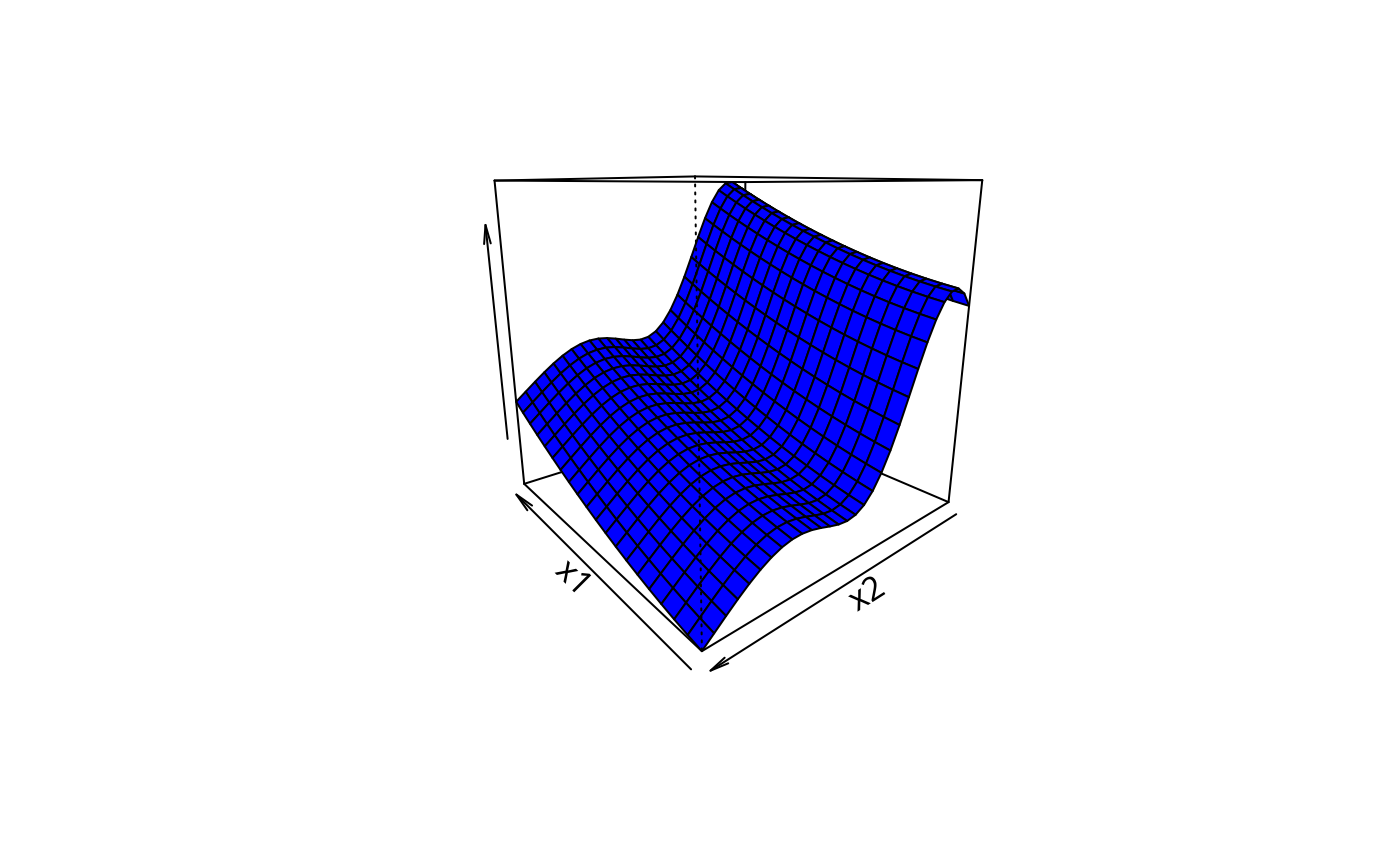
## custom perspective plot...
m1 <- 20;m2 <- 30; n <- m1*m2
x1 <- seq(.2,.8,length=m1);x2 <- seq(.2,.8,length=m2) ## marginal grid points
df <- data.frame(x0=rep(.5,n),x1=rep(x1,m2),x2=rep(x2,each=m1),x3=rep(0,n))
pf <- predict(b,newdata=df,type="terms")
persp(x1,x2,matrix(pf[,2]+pf[,3],m1,m2),theta=-130,col="blue",zlab="")
 #############################################
## difference between "terms" and "iterms"
#############################################
nd2 <- data.frame(x0=c(.25,.5),x1=c(.25,.5),x2=c(.25,.5),x3=c(.25,.5))
predict(b,nd2,type="terms",se=TRUE)
#> $fit
#> s(x0) s(I(x1^2)) s(x2)
#> 1 0.1642916 -1.4603275 5.7083123
#> 2 0.4032365 -0.3292994 -0.7451233
#>
#> $se.fit
#> s(x0) s(I(x1^2)) s(x2)
#> 1 0.1518415 0.12971641 0.3494252
#> 2 0.1650789 0.08963182 0.3197674
#>
#> attr(,"constant")
#> (Intercept)
#> 7.416319
predict(b,nd2,type="iterms",se=TRUE)
#> $fit
#> s(x0) s(I(x1^2)) s(x2)
#> 1 0.1642916 -1.4603275 5.7083123
#> 2 0.4032365 -0.3292994 -0.7451233
#>
#> $se.fit
#> s(x0) s(I(x1^2)) s(x2)
#> 1 0.2013941 0.1852839 0.3736332
#> 2 0.2115533 0.1598050 0.3460563
#>
#> attr(,"constant")
#> (Intercept)
#> 7.416319
#########################################################
## now get variance of sum of predictions using lpmatrix
#########################################################
Xp <- predict(b,newd,type="lpmatrix")
## Xp %*% coef(b) yields vector of predictions
a <- rep(1,31)
Xs <- t(a) %*% Xp ## Xs %*% coef(b) gives sum of predictions
var.sum <- Xs %*% b$Vp %*% t(Xs)
#############################################################
## Now get the variance of non-linear function of predictions
## by simulation from posterior distribution of the params
#############################################################
rmvn <- function(n,mu,sig) { ## MVN random deviates
L <- mroot(sig);m <- ncol(L);
t(mu + L%*%matrix(rnorm(m*n),m,n))
}
br <- rmvn(1000,coef(b),b$Vp) ## 1000 replicate param. vectors
res <- rep(0,1000)
for (i in 1:1000)
{ pr <- Xp %*% br[i,] ## replicate predictions
res[i] <- sum(log(abs(pr))) ## example non-linear function
}
mean(res);var(res)
#> [1] 58.85445
#> [1] 1.757425
## loop is replace-able by following ....
res <- colSums(log(abs(Xp %*% t(br))))
##################################################################
## The following shows how to use use an "lpmatrix" as a lookup
## table for approximate prediction. The idea is to create
## approximate prediction matrix rows by appropriate linear
## interpolation of an existing prediction matrix. The additivity
## of a GAM makes this possible.
## There is no reason to ever do this in R, but the following
## code provides a useful template for predicting from a fitted
## gam *outside* R: all that is needed is the coefficient vector
## and the prediction matrix. Use larger `Xp'/ smaller `dx' and/or
## higher order interpolation for higher accuracy.
###################################################################
xn <- c(.341,.122,.476,.981) ## want prediction at these values
x0 <- 1 ## intercept column
dx <- 1/30 ## covariate spacing in `newd'
for (j in 0:2) { ## loop through smooth terms
cols <- 1+j*9 +1:9 ## relevant cols of Xp
i <- floor(xn[j+1]*30) ## find relevant rows of Xp
w1 <- (xn[j+1]-i*dx)/dx ## interpolation weights
## find approx. predict matrix row portion, by interpolation
x0 <- c(x0,Xp[i+2,cols]*w1 + Xp[i+1,cols]*(1-w1))
}
dim(x0)<-c(1,28)
fv <- x0%*%coef(b) + xn[4];fv ## evaluate and add offset
#> [,1]
#> [1,] 6.385693
se <- sqrt(x0%*%b$Vp%*%t(x0));se ## get standard error
#> [,1]
#> [1,] 0.4356125
## compare to normal prediction
predict(b,newdata=data.frame(x0=xn[1],x1=xn[2],
x2=xn[3],x3=xn[4]),se=TRUE)
#> $fit
#> 1
#> 6.348329
#>
#> $se.fit
#> 1
#> 0.4438164
#>
##############################################################
## Example of producing a prediction interval for non Gaussian
## data...
##############################################################
f <- function(x) 0.2 * x^11 * (10 * (1 - x))^6 + 10 *
(10 * x)^3 * (1 - x)^10
set.seed(6);n <- 100;x <- sort(runif(n))
Ey <- exp(f(x)/4);scale <- .5
y <- rgamma(n,shape=1/scale,scale=Ey*scale) ## sim gamma dataexit
b <- gam(y~s(x,k=20),family=Gamma(link=log),method="REML")
Xp <- predict(b,type="lpmatrix")
br <- rmvn(10000,coef(b),vcov(b)) ## 1000 replicate param. vectors
fr <- Xp
yr <- apply(fr,2,function(x) rgamma(length(x),shape=1/b$scale,
scale=exp(x)*b$scale)) ## replicate data
pi <- apply(yr,1,quantile,probs=c(.1,.9),type=9) ## 80% PI
plot(x,y);lines(x,fitted(b));lines(x,pi[1,]);lines(x,pi[2,])
#############################################
## difference between "terms" and "iterms"
#############################################
nd2 <- data.frame(x0=c(.25,.5),x1=c(.25,.5),x2=c(.25,.5),x3=c(.25,.5))
predict(b,nd2,type="terms",se=TRUE)
#> $fit
#> s(x0) s(I(x1^2)) s(x2)
#> 1 0.1642916 -1.4603275 5.7083123
#> 2 0.4032365 -0.3292994 -0.7451233
#>
#> $se.fit
#> s(x0) s(I(x1^2)) s(x2)
#> 1 0.1518415 0.12971641 0.3494252
#> 2 0.1650789 0.08963182 0.3197674
#>
#> attr(,"constant")
#> (Intercept)
#> 7.416319
predict(b,nd2,type="iterms",se=TRUE)
#> $fit
#> s(x0) s(I(x1^2)) s(x2)
#> 1 0.1642916 -1.4603275 5.7083123
#> 2 0.4032365 -0.3292994 -0.7451233
#>
#> $se.fit
#> s(x0) s(I(x1^2)) s(x2)
#> 1 0.2013941 0.1852839 0.3736332
#> 2 0.2115533 0.1598050 0.3460563
#>
#> attr(,"constant")
#> (Intercept)
#> 7.416319
#########################################################
## now get variance of sum of predictions using lpmatrix
#########################################################
Xp <- predict(b,newd,type="lpmatrix")
## Xp %*% coef(b) yields vector of predictions
a <- rep(1,31)
Xs <- t(a) %*% Xp ## Xs %*% coef(b) gives sum of predictions
var.sum <- Xs %*% b$Vp %*% t(Xs)
#############################################################
## Now get the variance of non-linear function of predictions
## by simulation from posterior distribution of the params
#############################################################
rmvn <- function(n,mu,sig) { ## MVN random deviates
L <- mroot(sig);m <- ncol(L);
t(mu + L%*%matrix(rnorm(m*n),m,n))
}
br <- rmvn(1000,coef(b),b$Vp) ## 1000 replicate param. vectors
res <- rep(0,1000)
for (i in 1:1000)
{ pr <- Xp %*% br[i,] ## replicate predictions
res[i] <- sum(log(abs(pr))) ## example non-linear function
}
mean(res);var(res)
#> [1] 58.85445
#> [1] 1.757425
## loop is replace-able by following ....
res <- colSums(log(abs(Xp %*% t(br))))
##################################################################
## The following shows how to use use an "lpmatrix" as a lookup
## table for approximate prediction. The idea is to create
## approximate prediction matrix rows by appropriate linear
## interpolation of an existing prediction matrix. The additivity
## of a GAM makes this possible.
## There is no reason to ever do this in R, but the following
## code provides a useful template for predicting from a fitted
## gam *outside* R: all that is needed is the coefficient vector
## and the prediction matrix. Use larger `Xp'/ smaller `dx' and/or
## higher order interpolation for higher accuracy.
###################################################################
xn <- c(.341,.122,.476,.981) ## want prediction at these values
x0 <- 1 ## intercept column
dx <- 1/30 ## covariate spacing in `newd'
for (j in 0:2) { ## loop through smooth terms
cols <- 1+j*9 +1:9 ## relevant cols of Xp
i <- floor(xn[j+1]*30) ## find relevant rows of Xp
w1 <- (xn[j+1]-i*dx)/dx ## interpolation weights
## find approx. predict matrix row portion, by interpolation
x0 <- c(x0,Xp[i+2,cols]*w1 + Xp[i+1,cols]*(1-w1))
}
dim(x0)<-c(1,28)
fv <- x0%*%coef(b) + xn[4];fv ## evaluate and add offset
#> [,1]
#> [1,] 6.385693
se <- sqrt(x0%*%b$Vp%*%t(x0));se ## get standard error
#> [,1]
#> [1,] 0.4356125
## compare to normal prediction
predict(b,newdata=data.frame(x0=xn[1],x1=xn[2],
x2=xn[3],x3=xn[4]),se=TRUE)
#> $fit
#> 1
#> 6.348329
#>
#> $se.fit
#> 1
#> 0.4438164
#>
##############################################################
## Example of producing a prediction interval for non Gaussian
## data...
##############################################################
f <- function(x) 0.2 * x^11 * (10 * (1 - x))^6 + 10 *
(10 * x)^3 * (1 - x)^10
set.seed(6);n <- 100;x <- sort(runif(n))
Ey <- exp(f(x)/4);scale <- .5
y <- rgamma(n,shape=1/scale,scale=Ey*scale) ## sim gamma dataexit
b <- gam(y~s(x,k=20),family=Gamma(link=log),method="REML")
Xp <- predict(b,type="lpmatrix")
br <- rmvn(10000,coef(b),vcov(b)) ## 1000 replicate param. vectors
fr <- Xp
yr <- apply(fr,2,function(x) rgamma(length(x),shape=1/b$scale,
scale=exp(x)*b$scale)) ## replicate data
pi <- apply(yr,1,quantile,probs=c(.1,.9),type=9) ## 80% PI
plot(x,y);lines(x,fitted(b));lines(x,pi[1,]);lines(x,pi[2,])
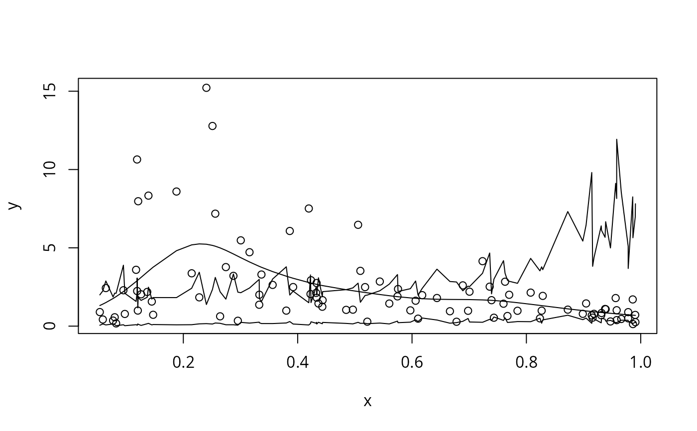 mean(y>pi[1,]&y<pi[2,]) ## check it
#> [1] 0.67
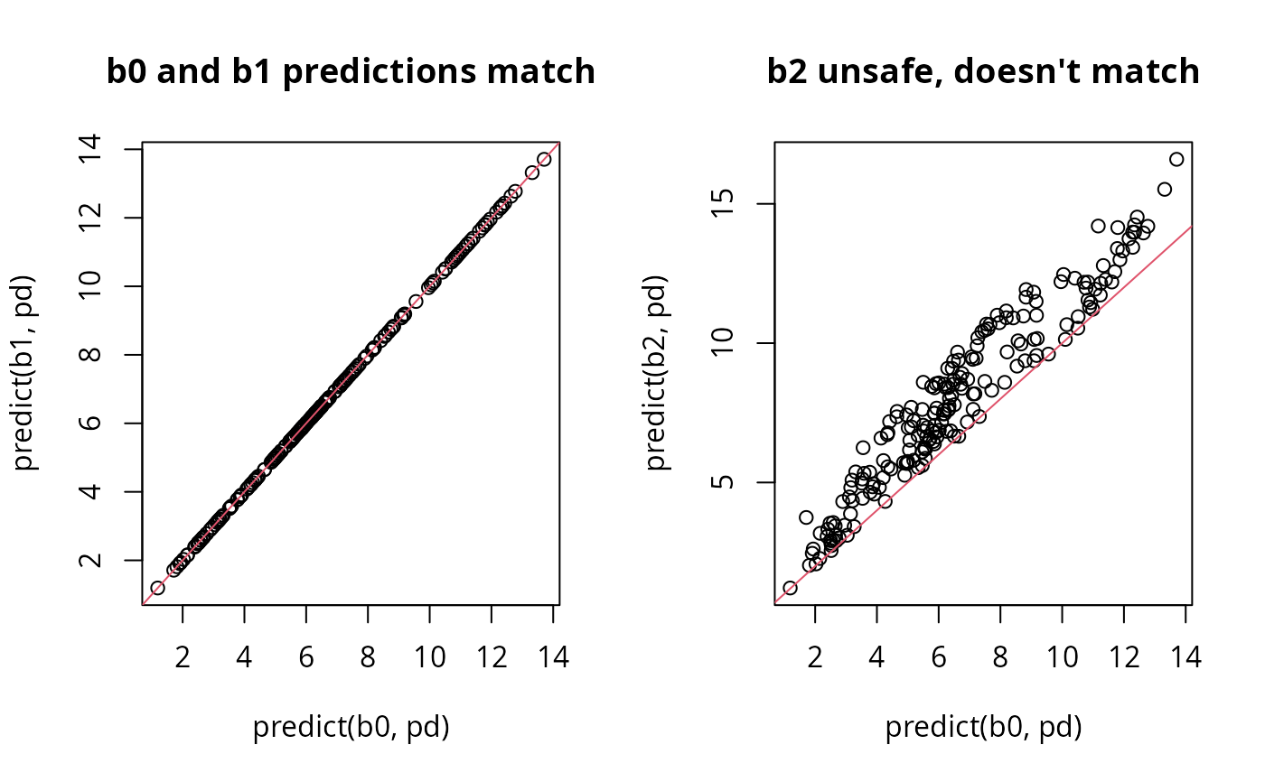
##################################################################
# illustration of unsafe scale dependent transforms in smooths....
##################################################################
b0 <- gam(y~s(x0)+s(x1)+s(x2)+x3,data=dat) ## safe
b1 <- gam(y~s(x0)+s(I(x1/2))+s(x2)+scale(x3),data=dat) ## safe
b2 <- gam(y~s(x0)+s(scale(x1))+s(x2)+scale(x3),data=dat) ## unsafe
pd <- dat; pd$x1 <- pd$x1/2; pd$x3 <- pd$x3/2
par(mfrow=c(1,2))
plot(predict(b0,pd),predict(b1,pd),main="b0 and b1 predictions match")
abline(0,1,col=2)
plot(predict(b0,pd),predict(b2,pd),main="b2 unsafe, doesn't match")
abline(0,1,col=2)
mean(y>pi[1,]&y<pi[2,]) ## check it
#> [1] 0.67
##################################################################
# illustration of unsafe scale dependent transforms in smooths....
##################################################################
b0 <- gam(y~s(x0)+s(x1)+s(x2)+x3,data=dat) ## safe
b1 <- gam(y~s(x0)+s(I(x1/2))+s(x2)+scale(x3),data=dat) ## safe
b2 <- gam(y~s(x0)+s(scale(x1))+s(x2)+scale(x3),data=dat) ## unsafe
pd <- dat; pd$x1 <- pd$x1/2; pd$x3 <- pd$x3/2
par(mfrow=c(1,2))
plot(predict(b0,pd),predict(b1,pd),main="b0 and b1 predictions match")
abline(0,1,col=2)
plot(predict(b0,pd),predict(b2,pd),main="b2 unsafe, doesn't match")
abline(0,1,col=2)
 ####################################################################
## Differentiating the smooths in a model (with CIs for derivatives)
####################################################################
## simulate data and fit model...
dat <- gamSim(1,n=300,scale=sig)
#> Gu & Wahba 4 term additive model
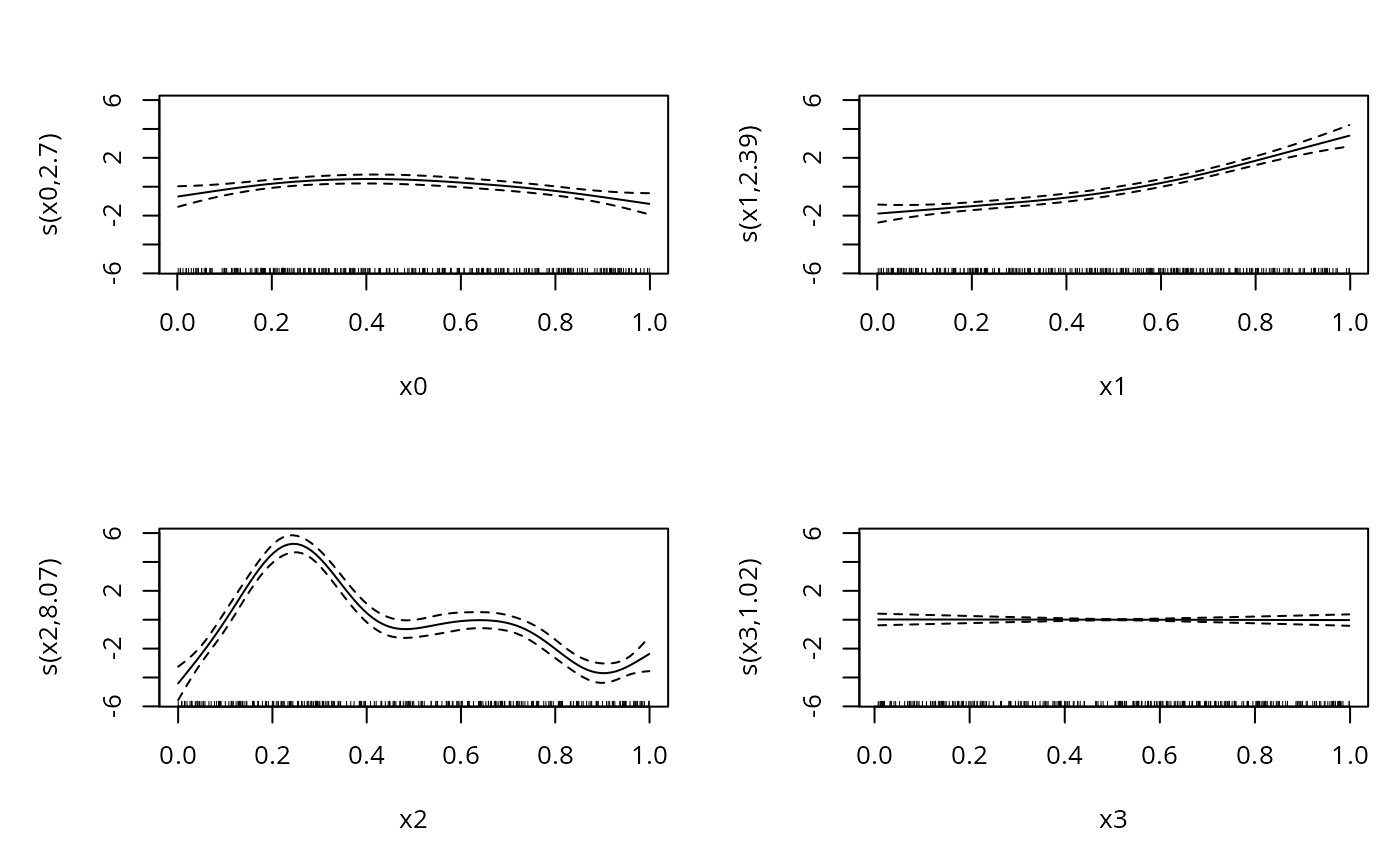
b<-gam(y~s(x0)+s(x1)+s(x2)+s(x3),data=dat)
plot(b,pages=1)
####################################################################
## Differentiating the smooths in a model (with CIs for derivatives)
####################################################################
## simulate data and fit model...
dat <- gamSim(1,n=300,scale=sig)
#> Gu & Wahba 4 term additive model
b<-gam(y~s(x0)+s(x1)+s(x2)+s(x3),data=dat)
plot(b,pages=1)
 ## now evaluate derivatives of smooths with associated standard
## errors, by finite differencing...
x.mesh <- seq(0,1,length=200) ## where to evaluate derivatives
newd <- data.frame(x0 = x.mesh,x1 = x.mesh, x2=x.mesh,x3=x.mesh)
X0 <- predict(b,newd,type="lpmatrix")
eps <- 1e-7 ## finite difference interval
x.mesh <- x.mesh + eps ## shift the evaluation mesh
newd <- data.frame(x0 = x.mesh,x1 = x.mesh, x2=x.mesh,x3=x.mesh)
X1 <- predict(b,newd,type="lpmatrix")
Xp <- (X1-X0)/eps ## maps coefficients to (fd approx.) derivatives
colnames(Xp) ## can check which cols relate to which smooth
#> [1] "(Intercept)" "s(x0).1" "s(x0).2" "s(x0).3" "s(x0).4"
#> [6] "s(x0).5" "s(x0).6" "s(x0).7" "s(x0).8" "s(x0).9"
#> [11] "s(x1).1" "s(x1).2" "s(x1).3" "s(x1).4" "s(x1).5"
#> [16] "s(x1).6" "s(x1).7" "s(x1).8" "s(x1).9" "s(x2).1"
#> [21] "s(x2).2" "s(x2).3" "s(x2).4" "s(x2).5" "s(x2).6"
#> [26] "s(x2).7" "s(x2).8" "s(x2).9" "s(x3).1" "s(x3).2"
#> [31] "s(x3).3" "s(x3).4" "s(x3).5" "s(x3).6" "s(x3).7"
#> [36] "s(x3).8" "s(x3).9"
par(mfrow=c(2,2))
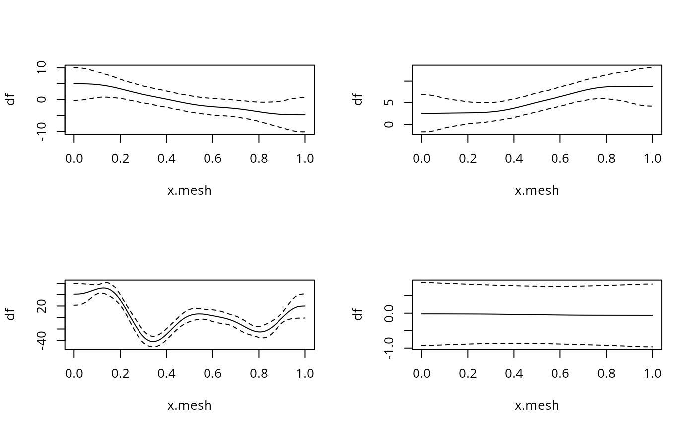
for (i in 1:4) { ## plot derivatives and corresponding CIs
Xi <- Xp*0
Xi[,(i-1)*9+1:9+1] <- Xp[,(i-1)*9+1:9+1] ## Xi%*%coef(b) = smooth deriv i
df <- Xi%*%coef(b) ## ith smooth derivative
df.sd <- rowSums(Xi%*%b$Vp*Xi)^.5 ## cheap diag(Xi%*%b$Vp%*%t(Xi))^.5
plot(x.mesh,df,type="l",ylim=range(c(df+2*df.sd,df-2*df.sd)))
lines(x.mesh,df+2*df.sd,lty=2);lines(x.mesh,df-2*df.sd,lty=2)
}
## now evaluate derivatives of smooths with associated standard
## errors, by finite differencing...
x.mesh <- seq(0,1,length=200) ## where to evaluate derivatives
newd <- data.frame(x0 = x.mesh,x1 = x.mesh, x2=x.mesh,x3=x.mesh)
X0 <- predict(b,newd,type="lpmatrix")
eps <- 1e-7 ## finite difference interval
x.mesh <- x.mesh + eps ## shift the evaluation mesh
newd <- data.frame(x0 = x.mesh,x1 = x.mesh, x2=x.mesh,x3=x.mesh)
X1 <- predict(b,newd,type="lpmatrix")
Xp <- (X1-X0)/eps ## maps coefficients to (fd approx.) derivatives
colnames(Xp) ## can check which cols relate to which smooth
#> [1] "(Intercept)" "s(x0).1" "s(x0).2" "s(x0).3" "s(x0).4"
#> [6] "s(x0).5" "s(x0).6" "s(x0).7" "s(x0).8" "s(x0).9"
#> [11] "s(x1).1" "s(x1).2" "s(x1).3" "s(x1).4" "s(x1).5"
#> [16] "s(x1).6" "s(x1).7" "s(x1).8" "s(x1).9" "s(x2).1"
#> [21] "s(x2).2" "s(x2).3" "s(x2).4" "s(x2).5" "s(x2).6"
#> [26] "s(x2).7" "s(x2).8" "s(x2).9" "s(x3).1" "s(x3).2"
#> [31] "s(x3).3" "s(x3).4" "s(x3).5" "s(x3).6" "s(x3).7"
#> [36] "s(x3).8" "s(x3).9"
par(mfrow=c(2,2))
for (i in 1:4) { ## plot derivatives and corresponding CIs
Xi <- Xp*0
Xi[,(i-1)*9+1:9+1] <- Xp[,(i-1)*9+1:9+1] ## Xi%*%coef(b) = smooth deriv i
df <- Xi%*%coef(b) ## ith smooth derivative
df.sd <- rowSums(Xi%*%b$Vp*Xi)^.5 ## cheap diag(Xi%*%b$Vp%*%t(Xi))^.5
plot(x.mesh,df,type="l",ylim=range(c(df+2*df.sd,df-2*df.sd)))
lines(x.mesh,df+2*df.sd,lty=2);lines(x.mesh,df-2*df.sd,lty=2)
}