Pairs Plot of compareFits Object
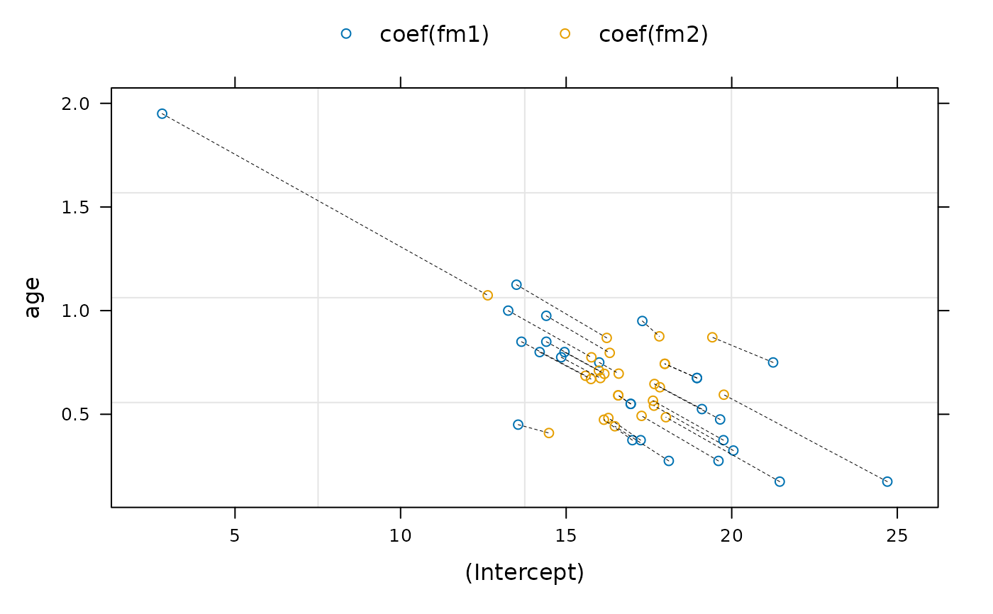
pairs.compareFits.RdScatter plots of the values being compared are generated for each pair
of coefficients in x. Different symbols (colors) are used
for each object being compared and values corresponding to the same
group are joined by a line, to facilitate comparison of fits. If only
two coefficients are present, the trellis function
xyplot is used; otherwise the trellis function splom
is used.
# S3 method for class 'compareFits'
pairs(x, subset, key, ...)
Arguments
- x
an object of class
compareFits.- subset
an optional logical or integer vector specifying which rows of
xshould be used in the plots. If missing, all rows are used.- key
an optional logical value, or list. If
TRUE, a legend is included at the top of the plot indicating which symbols (colors) correspond to which objects being compared. IfFALSE, no legend is included. If given as a list,keyis passed down as an argument to thetrellisfunction generating the plots (splomorxyplot). Defaults toTRUE.- ...
optional arguments passed down to the
trellisfunction generating the plots.
Value
Pairwise scatter plots of the values being compared, with different symbols (colors) used for each object under comparison.
See also
Examples
example(compareFits) # cF12 <- compareFits(coef(lmList(Orthodont)), .. lme(*))
#>
#> cmprFt> fm1 <- lmList(Orthodont)
#>
#> cmprFt> fm2 <- lme(fm1)
#>
#> cmprFt> (cF12 <- compareFits(coef(fm1), coef(fm2)))
#> , , (Intercept)
#>
#>     coef(fm1) coef(fm2)
#> M16     16.95  16.57335
#> M05     13.65  15.58444
#> M02     14.85  16.03361
#> M11     20.05  17.65160
#> M07     14.95  16.15314
#> M08     19.75  17.62141
#> M03     16.00  16.58721
#> M12     13.25  15.76312
#> M13      2.80  12.63156
#> M14     19.10  17.66546
#> M09     14.40  16.31671
#> M15     13.50  16.22614
#> M06     18.95  17.97875
#> M04     24.70  19.76157
#> M01     17.30  17.81269
#> M10     21.25  19.41435
#> F10     13.55  14.47973
#> F09     18.10  16.47016
#> F06     17.00  16.14053
#> F01     17.25  16.27515
#> F05     19.60  17.27792
#> F07     16.95  16.57335
#> F02     14.20  15.74926
#> F08     21.45  18.01143
#> F03     14.40  15.98832
#> F04     19.65  17.83028
#> F11     18.95  17.97875
#>
#> , , age
#>
#>     coef(fm1) coef(fm2)
#> M16     0.550 0.5913314
#> M05     0.850 0.6857856
#> M02     0.775 0.6746931
#> M11     0.325 0.5413591
#> M07     0.800 0.6950853
#> M08     0.375 0.5654488
#> M03     0.750 0.6960376
#> M12     1.000 0.7747494
#> M13     1.950 1.0738543
#> M14     0.525 0.6460653
#> M09     0.975 0.7960939
#> M15     1.125 0.8683630
#> M06     0.675 0.7433764
#> M04     0.175 0.5943001
#> M01     0.950 0.8758698
#> M10     0.750 0.8713317
#> F10     0.450 0.4095945
#> F09     0.275 0.4421434
#> F06     0.375 0.4736281
#> F01     0.375 0.4819754
#> F05     0.275 0.4922274
#> F07     0.550 0.5913314
#> F02     0.800 0.6700432
#> F08     0.175 0.4857847
#> F03     0.850 0.7108276
#> F04     0.475 0.6303229
#> F11     0.675 0.7433764
#>
pairs(cF12)