Plot a compareFits Object
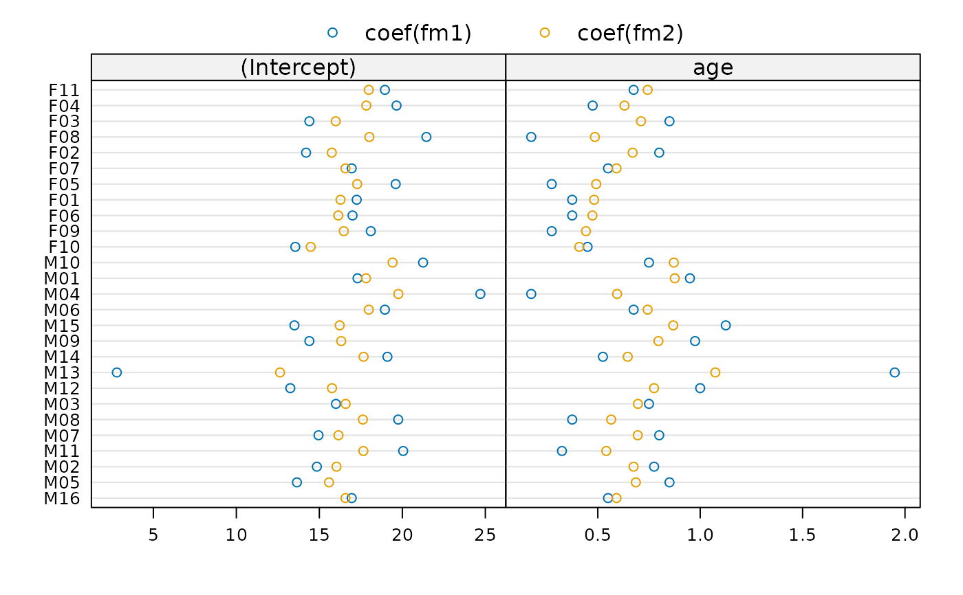
plot.compareFits.RdA Trellis dotplot of the values being compared, with different
rows per group, is generated, with a different panel for each
coefficient. Different symbols (colors) are used for each object being
compared.
# S3 method for class 'compareFits'
plot(x, subset, key, mark, ...)
Arguments
- x
an object of class
"compareFits".- subset
an optional logical or integer vector specifying which rows of
xshould be used in the plots. If missing, all rows are used.- key
an optional logical value, or list. If
TRUE, a legend is included at the top of the plot indicating which symbols (colors) correspond to which objects being compared. IfFALSE, no legend is included. If given as a list,keyis passed down as an argument to thetrellisfunction generating the plots (dotplot). Defaults toTRUE.- mark
an optional numeric vector, of length equal to the number of coefficients being compared, indicating where vertical lines should be drawn in the plots. If missing, no lines are drawn.
- ...
optional arguments passed down to the
trellisfunction generating the plots.
Value
A Trellis dotplot of the values being compared, with rows
determined by the groups and panels by the coefficients.
See also
Examples
example(compareFits) # cF12 <- compareFits(coef(lmList(Orthodont)), .. lme(*))
#>
#> cmprFt> fm1 <- lmList(Orthodont)
#>
#> cmprFt> fm2 <- lme(fm1)
#>
#> cmprFt> (cF12 <- compareFits(coef(fm1), coef(fm2)))
#> , , (Intercept)
#>
#>     coef(fm1) coef(fm2)
#> M16     16.95  16.57335
#> M05     13.65  15.58444
#> M02     14.85  16.03361
#> M11     20.05  17.65160
#> M07     14.95  16.15314
#> M08     19.75  17.62141
#> M03     16.00  16.58721
#> M12     13.25  15.76312
#> M13      2.80  12.63156
#> M14     19.10  17.66546
#> M09     14.40  16.31671
#> M15     13.50  16.22614
#> M06     18.95  17.97875
#> M04     24.70  19.76157
#> M01     17.30  17.81269
#> M10     21.25  19.41435
#> F10     13.55  14.47973
#> F09     18.10  16.47016
#> F06     17.00  16.14053
#> F01     17.25  16.27515
#> F05     19.60  17.27792
#> F07     16.95  16.57335
#> F02     14.20  15.74926
#> F08     21.45  18.01143
#> F03     14.40  15.98832
#> F04     19.65  17.83028
#> F11     18.95  17.97875
#>
#> , , age
#>
#>     coef(fm1) coef(fm2)
#> M16     0.550 0.5913314
#> M05     0.850 0.6857856
#> M02     0.775 0.6746931
#> M11     0.325 0.5413591
#> M07     0.800 0.6950853
#> M08     0.375 0.5654488
#> M03     0.750 0.6960376
#> M12     1.000 0.7747494
#> M13     1.950 1.0738543
#> M14     0.525 0.6460653
#> M09     0.975 0.7960939
#> M15     1.125 0.8683630
#> M06     0.675 0.7433764
#> M04     0.175 0.5943001
#> M01     0.950 0.8758698
#> M10     0.750 0.8713317
#> F10     0.450 0.4095945
#> F09     0.275 0.4421434
#> F06     0.375 0.4736281
#> F01     0.375 0.4819754
#> F05     0.275 0.4922274
#> F07     0.550 0.5913314
#> F02     0.800 0.6700432
#> F08     0.175 0.4857847
#> F03     0.850 0.7108276
#> F04     0.475 0.6303229
#> F11     0.675 0.7433764
#>
plot(cF12)