Working with multiple endpoints
2025-09-05
Source:vignettes/multiple-endpoints.Rmd
multiple-endpoints.RmdMultiple endpoints
Joint PK/PD models, or PK/PD models where you fix certain components are common in pharmacometrics. A classic example, (provided by Tomoo Funaki and Nick Holford) is Warfarin.
In this example, we have a transit-compartment (from depot to gut to central volume) PK model and an effect compartment for the PCA measurement.
Below is an illustrated example of a model that can be applied to the data:
pk.turnover.emax <- function() {
  ini({
    tktr <- log(1)
    tka <- log(1)
    tcl <- log(0.1)
    tv <- log(10)
    ##
    eta.ktr ~ 1
    eta.ka ~ 1
    eta.cl ~ 2
    eta.v ~ 1
    prop.err <- 0.1
    pkadd.err <- 0.1
    ##
    temax <- logit(0.8)
    #temax <- 7.5
    tec50 <- log(0.5)
    tkout <- log(0.05)
    te0 <- log(100)
    ##
    eta.emax ~ .5
    eta.ec50  ~ .5
    eta.kout ~ .5
    eta.e0 ~ .5
    ##
    pdadd.err <- 10
  })
  model({
    ktr <- exp(tktr + eta.ktr)
    ka <- exp(tka + eta.ka)
    cl <- exp(tcl + eta.cl)
    v <- exp(tv + eta.v)
    ##
    #poplogit = log(temax/(1-temax))
    emax=expit(temax+eta.emax)
    #logit=temax+eta.emax
    ec50 =  exp(tec50 + eta.ec50)
    kout = exp(tkout + eta.kout)
    e0 = exp(te0 + eta.e0)
    ##
    DCP = center/v
    PD=1-emax*DCP/(ec50+DCP)
    ##
    effect(0) = e0
    kin = e0*kout
    ##
    d/dt(depot) = -ktr * depot
    d/dt(gut) =  ktr * depot -ka * gut
    d/dt(center) =  ka * gut - cl / v * center
    d/dt(effect) = kin*PD -kout*effect
    ##
    cp = center / v
    cp ~ prop(prop.err) + add(pkadd.err)
    effect ~ add(pdadd.err)
  })
}
Notice there are two endpoints in the model cp and
effect. Both are modeled in nlmixr using the ~
“modeled by” specification.
To see more about how nlmixr will handle the multiple compartment model, it is quite informative to parse the model and print the information about that model. In this case an initial parsing would give:
ui <- nlmixr(pk.turnover.emax)
uiIn the middle of the printout, it shows how the data must be
formatted (using the cmt and dvid data items)
to allow nlmixr to model the multiple endpoint appropriately.
Of course, if you are interested you can directly access the
information in ui$multipleEndpoint.
ui$multipleEndpoint
#>     variable                   cmt                   dvid*
#> 1     cp ~ …     cmt='cp' or cmt=5     dvid='cp' or dvid=1
#> 2 effect ~ … cmt='effect' or cmt=4 dvid='effect' or dvid=2
Notice that the cmt and dvid items can use
the named variables directly as either the cmt or
dvid specification. This flexible notation makes it so you
do not have to rename your compartments to run nlmixr model
functions.
The other thing to note is that the cp is specified by
an ODE compartment above the number of compartments defined in the
rxode2 part of the nlmixr model. This is
because cp is not a defined compartment, but a related
variable cp.
The last thing to notice that the cmt items are numbered
cmt=5 for cp or cmt=4 for
effect even though they were specified in the model first
by cp and cmt. This ordering is because
effect is a compartment in the rxode2 system.
Of course cp is related to the compartment
center, and it may make more sense to pair cp
with the center compartment.
If this is something you want to have you can specify the compartment
to relate the effect to by the | operator. In this case you
would change
cp ~ prop(prop.err) + add(pkadd.err)to
cp ~ prop(prop.err) + add(pkadd.err) | centerWith this change, the model could be updated to:
pk.turnover.emax2 <- function() {
  ini({
    tktr <- log(1)
    tka <- log(1)
    tcl <- log(0.1)
    tv <- log(10)
    ##
    eta.ktr ~ 1
    eta.ka ~ 1
    eta.cl ~ 2
    eta.v ~ 1
    prop.err <- 0.1
    pkadd.err <- 0.1
    ##
    temax <- logit(0.8)
    tec50 <- log(0.5)
    tkout <- log(0.05)
    te0 <- log(100)
    ##
    eta.emax ~ .5
    eta.ec50  ~ .5
    eta.kout ~ .5
    eta.e0 ~ .5
    ##
    pdadd.err <- 10
  })
  model({
    ktr <- exp(tktr + eta.ktr)
    ka <- exp(tka + eta.ka)
    cl <- exp(tcl + eta.cl)
    v <- exp(tv + eta.v)
    ##
    emax=expit(temax+eta.emax)
    ec50 =  exp(tec50 + eta.ec50)
    kout = exp(tkout + eta.kout)
    e0 = exp(te0 + eta.e0)
    ##
    DCP = center/v
    PD=1-emax*DCP/(ec50+DCP)
    ##
    effect(0) = e0
    kin = e0*kout
    ##
    d/dt(depot) = -ktr * depot
    d/dt(gut) =  ktr * depot -ka * gut
    d/dt(center) =  ka * gut - cl / v * center
    d/dt(effect) = kin*PD -kout*effect
    ##
    cp = center / v
    cp ~ prop(prop.err) + add(pkadd.err) | center
    effect ~ add(pdadd.err)
  })
}
ui2 <- nlmixr(pk.turnover.emax2)
ui2$multipleEndpoint
#>     variable                   cmt                   dvid*
#> 1     cp ~ … cmt='center' or cmt=3 dvid='center' or dvid=1
#> 2 effect ~ … cmt='effect' or cmt=4 dvid='effect' or dvid=2
Notice in this case the cmt variables are numbered
sequentially and the cp variable matches the
center compartment.
DVID vs CMT, which one is used
When dvid and cmt are combined in the same
dataset, the cmt data item is always used on the event
information and the dvid is used on the observations.
nlmixr expects the cmt data item to match the
dvid item for observations OR to be either zero or one for
the dvid to replace the cmt information.
If you do not wish to use dvid items to define multiple
endpoints in nlmixr, you can set the following option:
options(rxode2.combine.dvid=FALSE)
ui2$multipleEndpoint
#>     variable                   cmt
#> 1     cp ~ … cmt='center' or cmt=3
#> 2 effect ~ … cmt='effect' or cmt=4
Then only cmt items are used for the multiple endpoint
models. Of course you can turn it on or off for different models if you
wish:
options(rxode2.combine.dvid=TRUE)
ui2$multipleEndpoint
#>     variable                   cmt                   dvid*
#> 1     cp ~ … cmt='center' or cmt=3 dvid='center' or dvid=1
#> 2 effect ~ … cmt='effect' or cmt=4 dvid='effect' or dvid=2
Running a multiple endpoint model
With this information, we can use the built-in warfarin dataset in
nlmixr2:
summary(warfarin)
#>        id             time             amt                dv          dvid
#>  Min.   : 1.00   Min.   :  0.00   Min.   :  0.000   Min.   :  0.00   cp :283
#>  1st Qu.: 8.00   1st Qu.: 24.00   1st Qu.:  0.000   1st Qu.:  4.50   pca:232
#>  Median :15.00   Median : 48.00   Median :  0.000   Median : 11.40
#>  Mean   :16.08   Mean   : 52.08   Mean   :  6.524   Mean   : 20.02
#>  3rd Qu.:24.00   3rd Qu.: 96.00   3rd Qu.:  0.000   3rd Qu.: 26.00
#>  Max.   :33.00   Max.   :144.00   Max.   :153.000   Max.   :100.00
#>       evid               wt              age            sex
#>  Min.   :0.00000   Min.   : 40.00   Min.   :21.00   female:101
#>  1st Qu.:0.00000   1st Qu.: 60.00   1st Qu.:23.00   male  :414
#>  Median :0.00000   Median : 70.00   Median :28.00
#>  Mean   :0.06214   Mean   : 69.27   Mean   :31.85
#>  3rd Qu.:0.00000   3rd Qu.: 78.00   3rd Qu.:36.00
#>  Max.   :1.00000   Max.   :102.00   Max.   :63.00
Since dvid specifies pca as the effect endpoint, you can
update the model to be more explicit making one last change:
cp ~ prop(prop.err) + add(pkadd.err)
effect ~ add(pdadd.err)
to
cp ~ prop(prop.err) + add(pkadd.err)
effect ~ add(pdadd.err)  | pca
pk.turnover.emax3 <- function() {
  ini({
    tktr <- log(1)
    tka <- log(1)
    tcl <- log(0.1)
    tv <- log(10)
    ##
    eta.ktr ~ 1
    eta.ka ~ 1
    eta.cl ~ 2
    eta.v ~ 1
    prop.err <- 0.1
    pkadd.err <- 0.1
    ##
    temax <- logit(0.8)
    tec50 <- log(0.5)
    tkout <- log(0.05)
    te0 <- log(100)
    ##
    eta.emax ~ .5
    eta.ec50  ~ .5
    eta.kout ~ .5
    eta.e0 ~ .5
    ##
    pdadd.err <- 10
  })
  model({
    ktr <- exp(tktr + eta.ktr)
    ka <- exp(tka + eta.ka)
    cl <- exp(tcl + eta.cl)
    v <- exp(tv + eta.v)
    emax = expit(temax+eta.emax)
    ec50 =  exp(tec50 + eta.ec50)
    kout = exp(tkout + eta.kout)
    e0 = exp(te0 + eta.e0)
    ##
    DCP = center/v
    PD=1-emax*DCP/(ec50+DCP)
    ##
    effect(0) = e0
    kin = e0*kout
    ##
    d/dt(depot) = -ktr * depot
    d/dt(gut) =  ktr * depot -ka * gut
    d/dt(center) =  ka * gut - cl / v * center
    d/dt(effect) = kin*PD -kout*effect
    ##
    cp = center / v
    cp ~ prop(prop.err) + add(pkadd.err)
    effect ~ add(pdadd.err) | pca
  })
}
Run the models with SAEM
fit.TOS <- nlmixr(pk.turnover.emax3, warfarin, "saem", control=list(print=0),
table=list(cwres=TRUE, npde=TRUE))
#> [====|====|====|====|====|====|====|====|====|====] 0:00:00
#> [====|====|====|====|====|====|====|====|====|====] 0:00:00
print(fit.TOS)
#> ── nlmixr² SAEM OBJF by FOCEi approximation ──
#>
#> OBJF AIC BIC Log-likelihood Condition#(Cov) Condition#(Cor)
#> FOCEi 1384.304 2309.999 2389.419 -1135.999 3888.244 22.06544
#>
#> ── Time (sec $time): ──
#>
#> setup optimize covariance saem table compress
#> elapsed 0.002756 9e-06 0.066019 120.142 17.552 0.023
#>
#> ── Population Parameters ($parFixed or $parFixedDf): ──
#>
#> Est. SE %RSE Back-transformed(95%CI) BSV(CV% or SD)
#> tktr 0.44 0.529 120 1.55 (0.55, 4.38) 110.
#> tka -0.261 0.269 103 0.77 (0.455, 1.3) 13.5
#> tcl -1.97 0.0515 2.62 0.14 (0.126, 0.155) 26.8
#> tv 2.01 0.0484 2.41 7.43 (6.76, 8.17) 21.8
#> prop.err 0.12 0.12
#> pkadd.err 0.805 0.805
#> temax 3.44 0.696 20.2 0.969 (0.888, 0.992) 0.251
#> tec50 -0.094 0.146 155 0.91 (0.684, 1.21) 45.9
#> tkout -2.94 0.0384 1.31 0.0531 (0.0492, 0.0572) 5.99
#> te0 4.57 0.0115 0.253 96.6 (94.4, 98.8) 5.29
#> pdadd.err 3.6 3.6
#> Shrink(SD)%
#> tktr 44.4%
#> tka 81.5%
#> tcl 6.80%
#> tv 15.9%
#> prop.err
#> pkadd.err
#> temax 81.1%
#> tec50 9.86%
#> tkout 45.4%
#> te0 17.0%
#> pdadd.err
#>
#> Covariance Type ($covMethod): linFim
#> No correlations in between subject variability (BSV) matrix
#> Full BSV covariance ($omega) or correlation ($omegaR; diagonals=SDs)
#> Distribution stats (mean/skewness/kurtosis/p-value) available in $shrink
#> Censoring ($censInformation): No censoring
#>
#> ── Fit Data (object is a modified tibble): ──
#> # A tibble: 483 × 44
#> ID TIME CMT DV EPRED ERES NPDE NPD PDE PD PRED RES
#> <fct> <dbl> <fct> <dbl> <dbl> <dbl> <dbl> <dbl> <dbl> <dbl> <dbl> <dbl>
#> 1 1 0.5 cp 0 1.76 -1.76 -1.79 -1.50 0.0367 0.0667 1.38 -1.38
#> 2 1 1 cp 1.9 4.06 -2.16 1.75 -0.954 0.96 0.17 3.87 -1.97
#> 3 1 2 cp 3.3 7.93 -4.63 -1.99 -1.71 0.0233 0.0433 8.18 -4.88
#> # ℹ 480 more rows
#> # ℹ 32 more variables: WRES <dbl>, IPRED <dbl>, IRES <dbl>, IWRES <dbl>,
#> # CPRED <dbl>, CRES <dbl>, CWRES <dbl>, eta.ktr <dbl>, eta.ka <dbl>,
#> # eta.cl <dbl>, eta.v <dbl>, eta.emax <dbl>, eta.ec50 <dbl>, eta.kout <dbl>,
#> # eta.e0 <dbl>, depot <dbl>, gut <dbl>, center <dbl>, effect <dbl>,
#> # ktr <dbl>, ka <dbl>, cl <dbl>, v <dbl>, emax <dbl>, ec50 <dbl>, kout <dbl>,
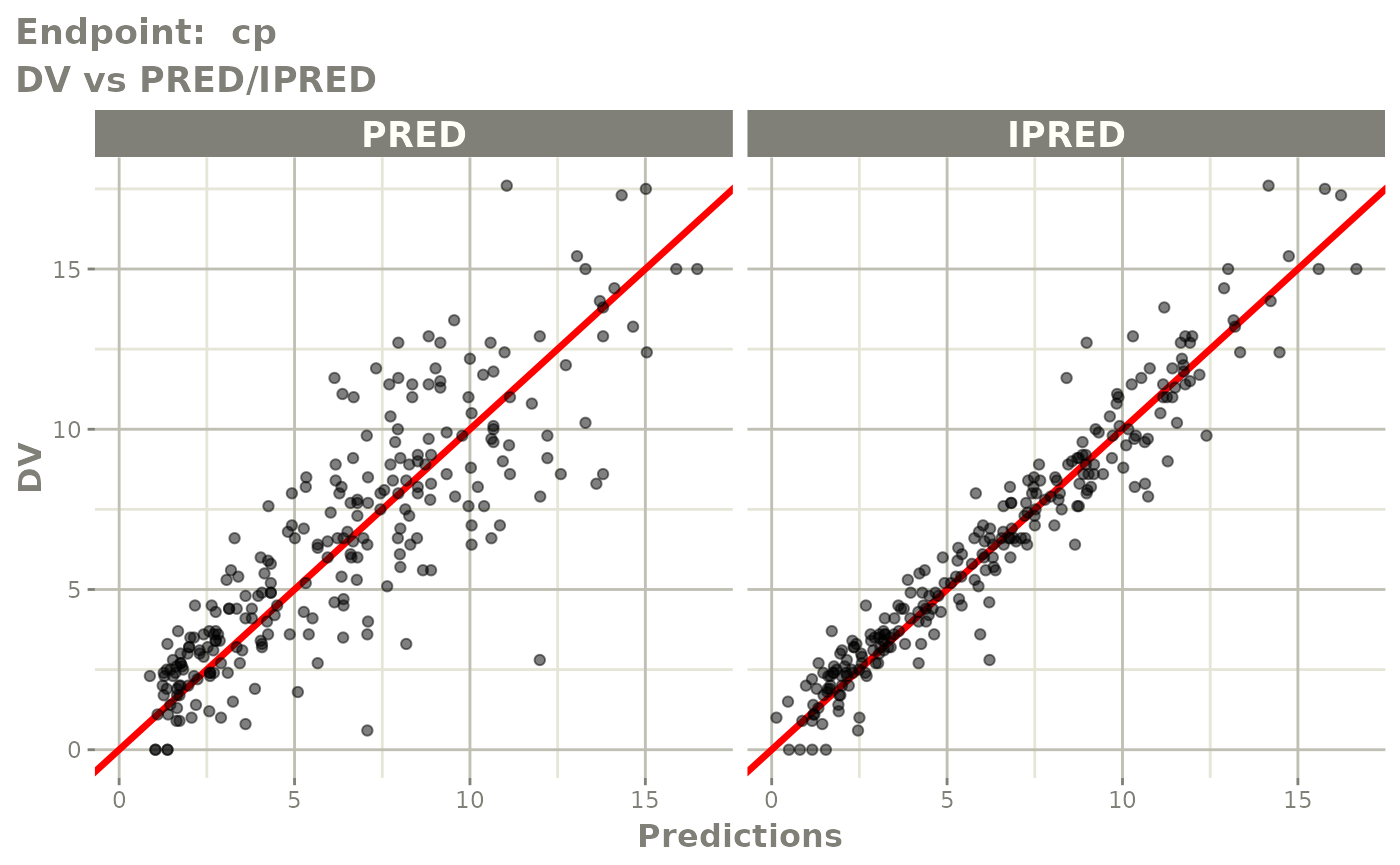
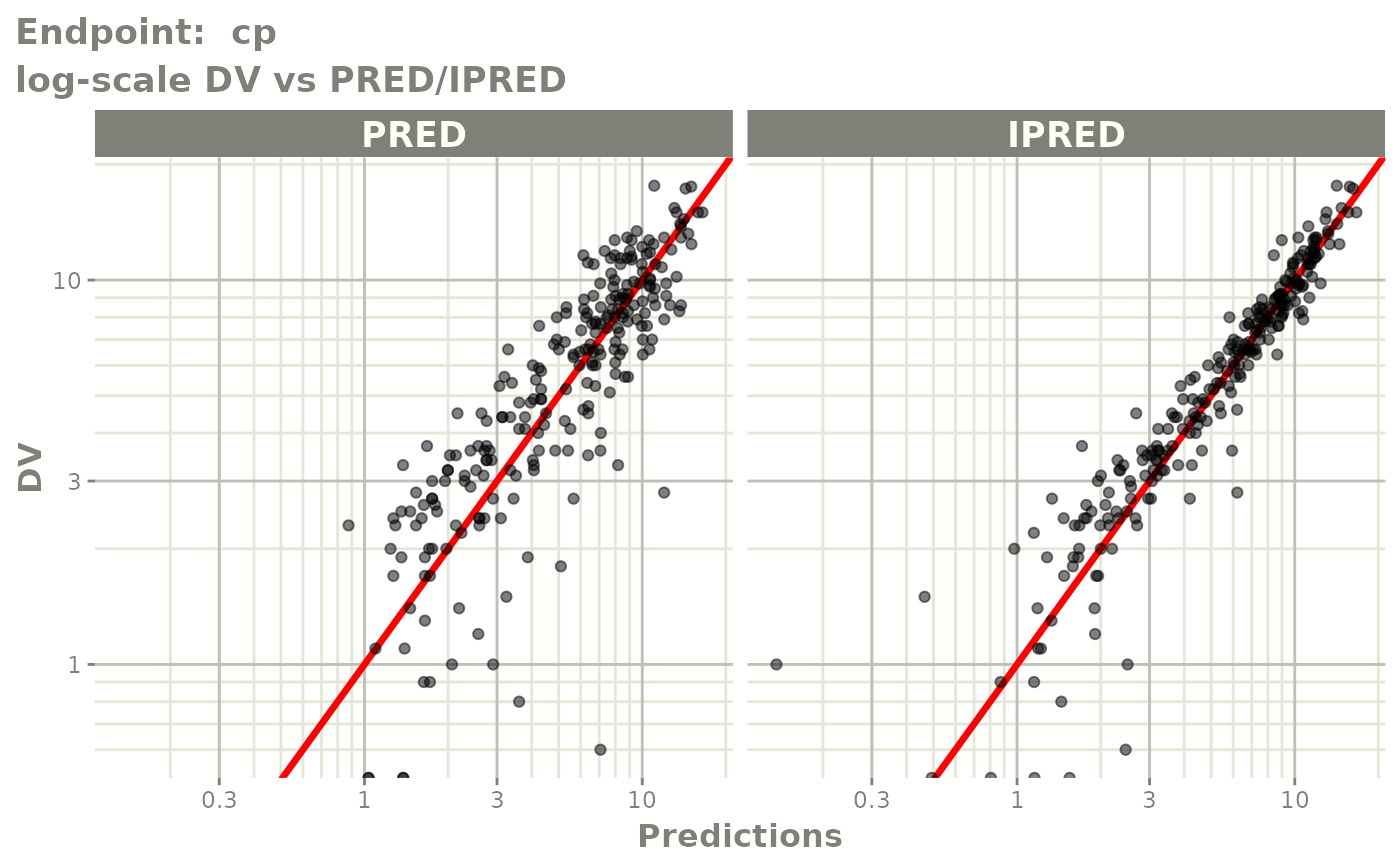
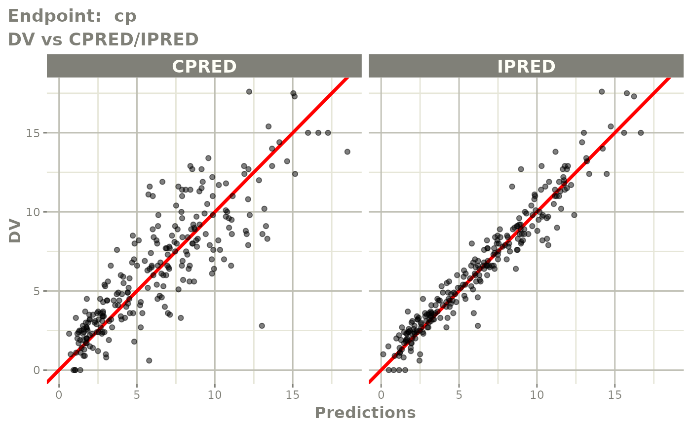
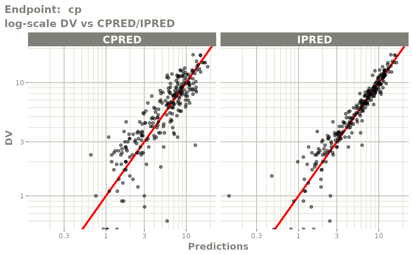
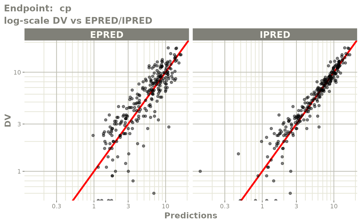
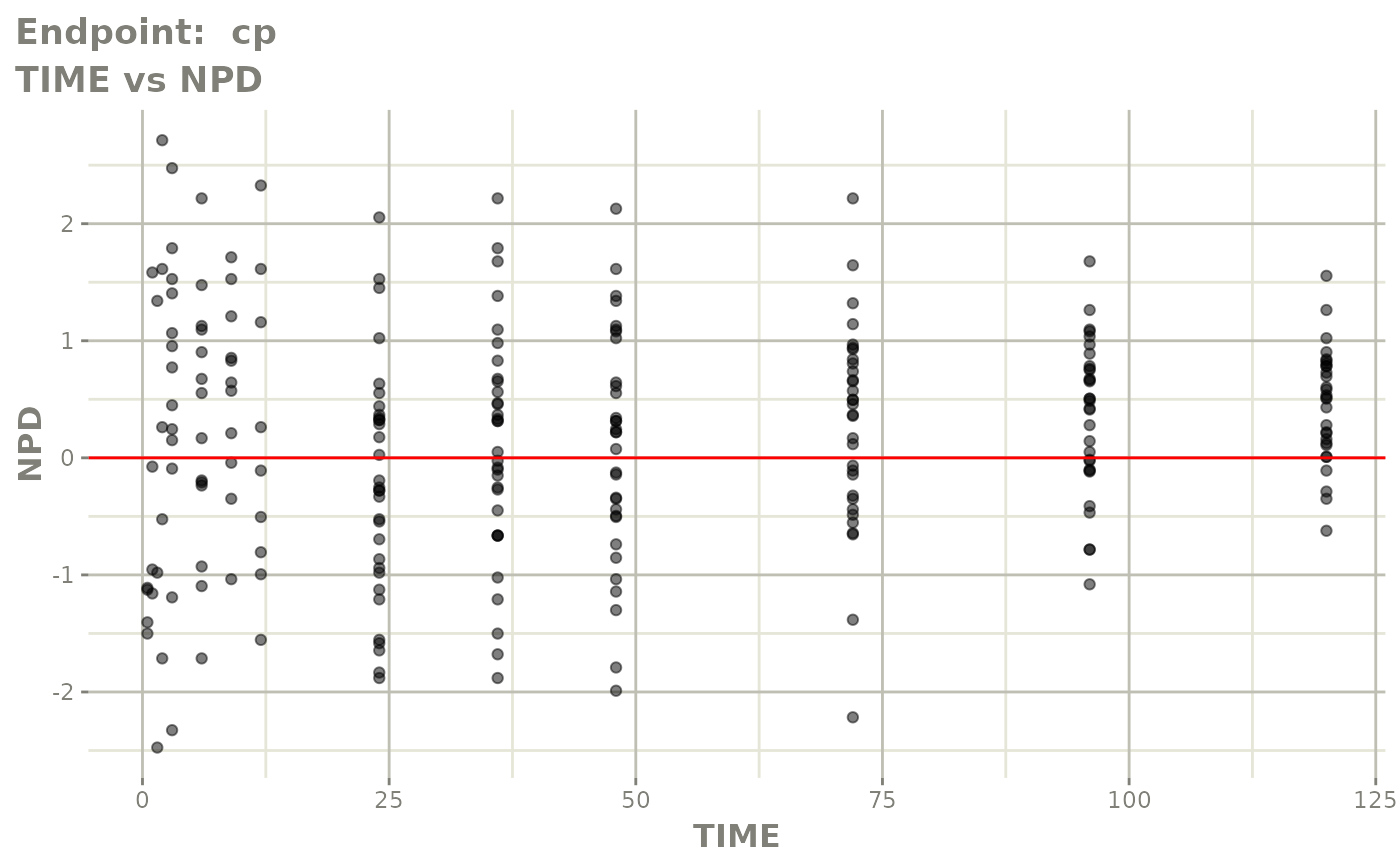
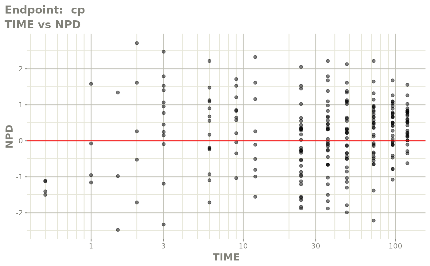
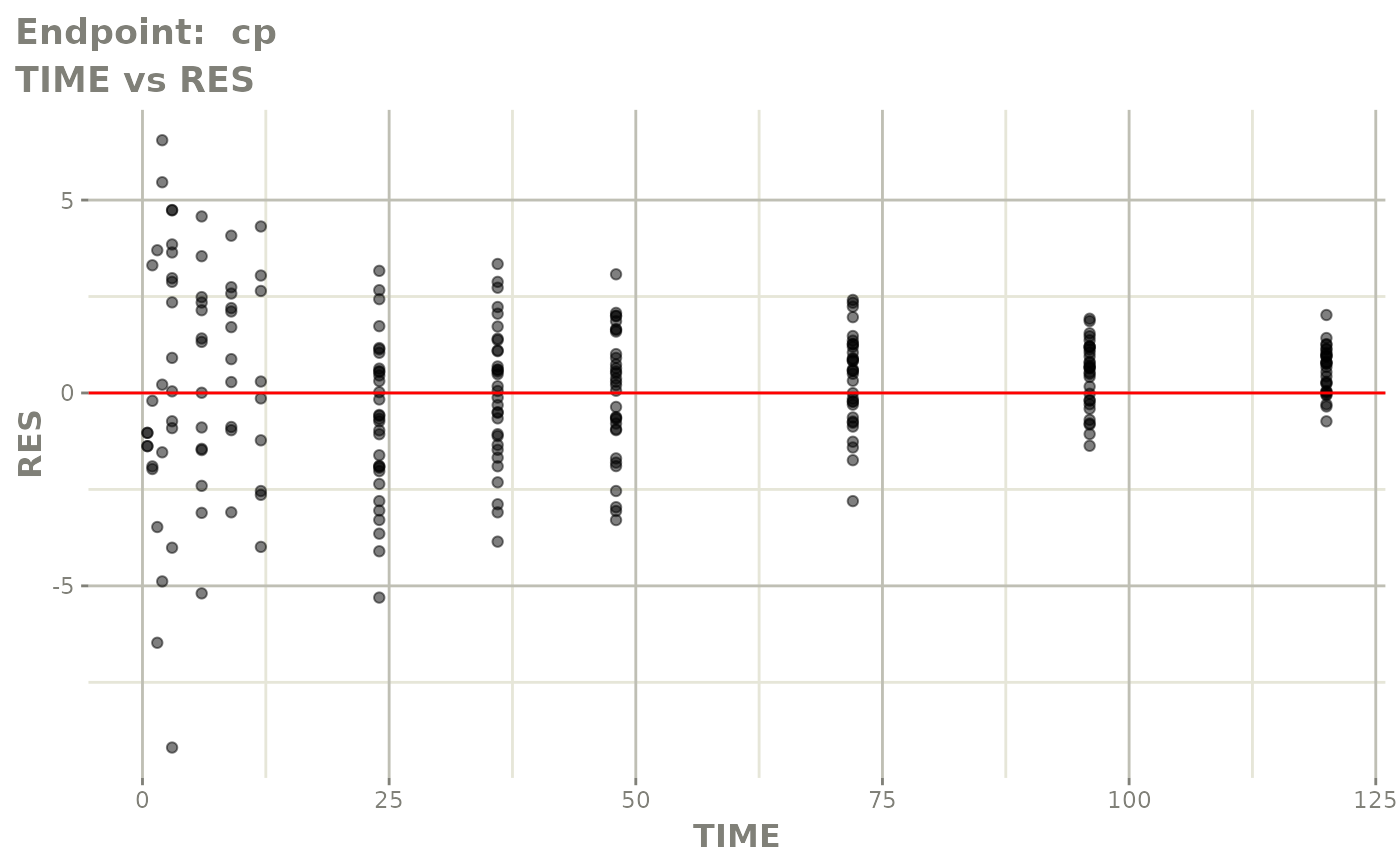
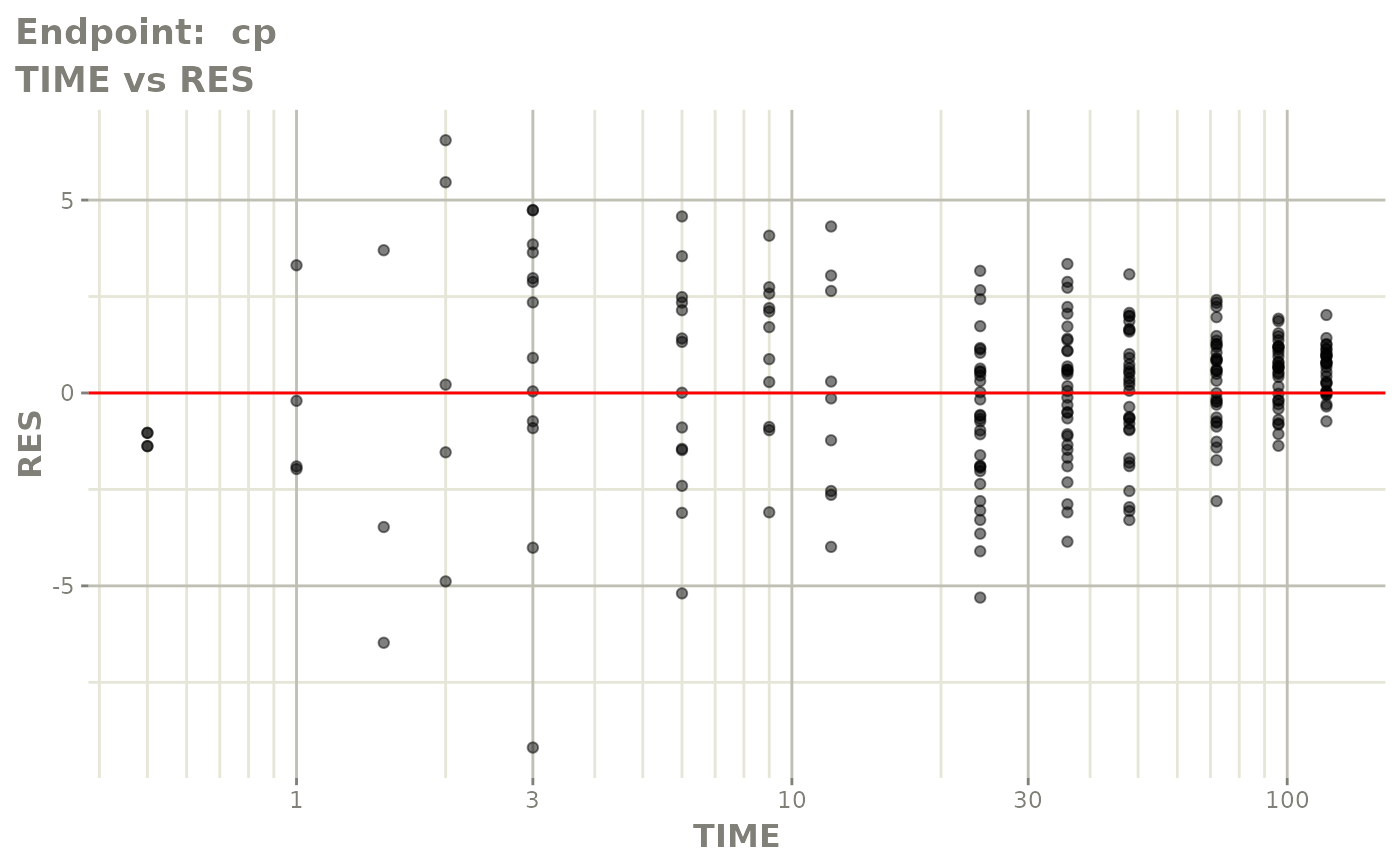
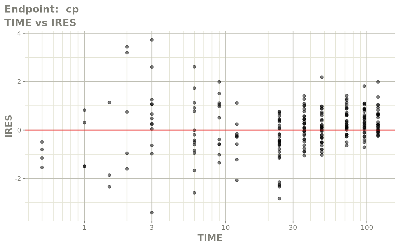
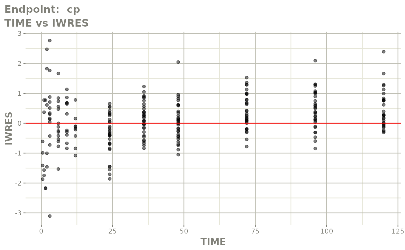
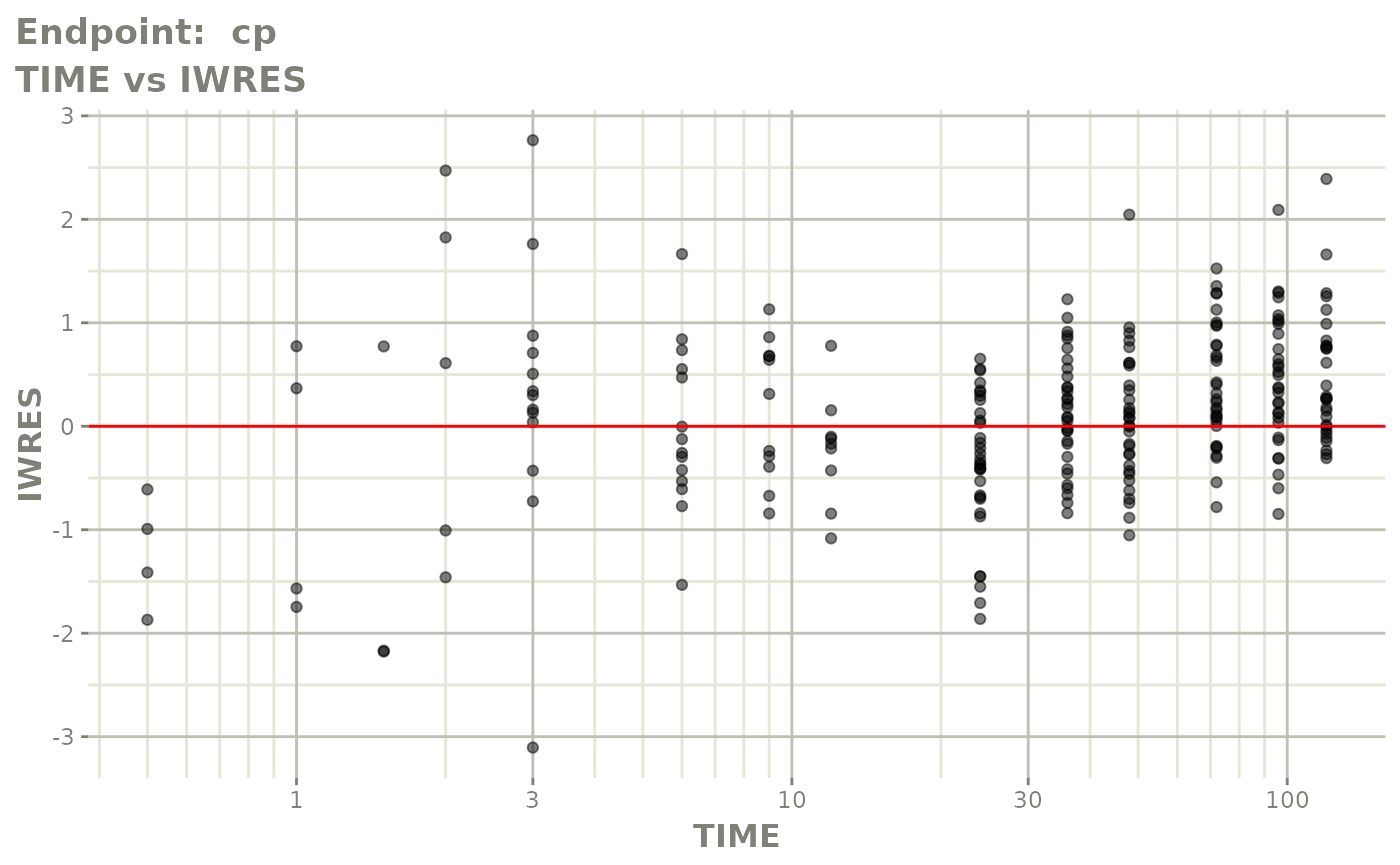
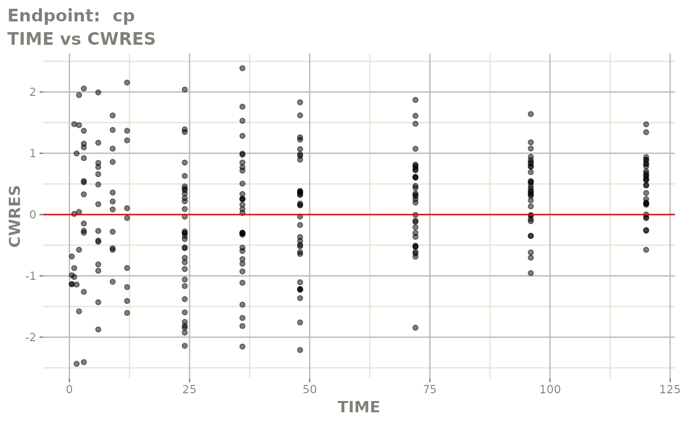
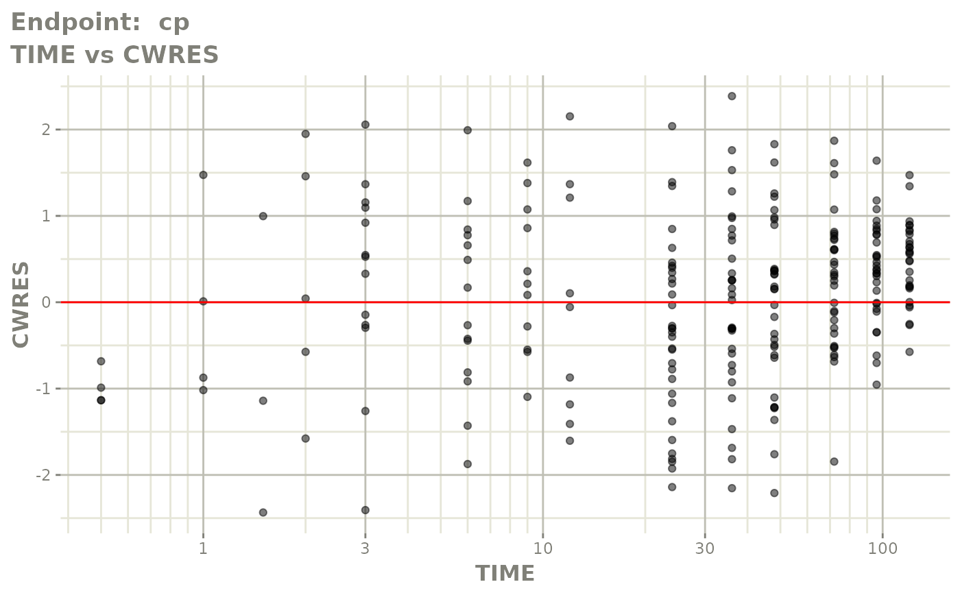
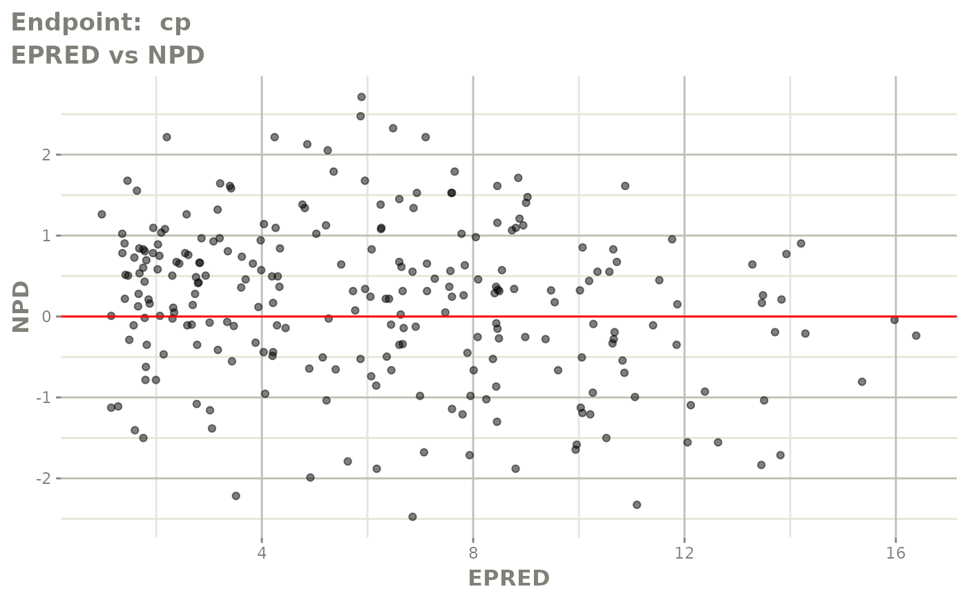
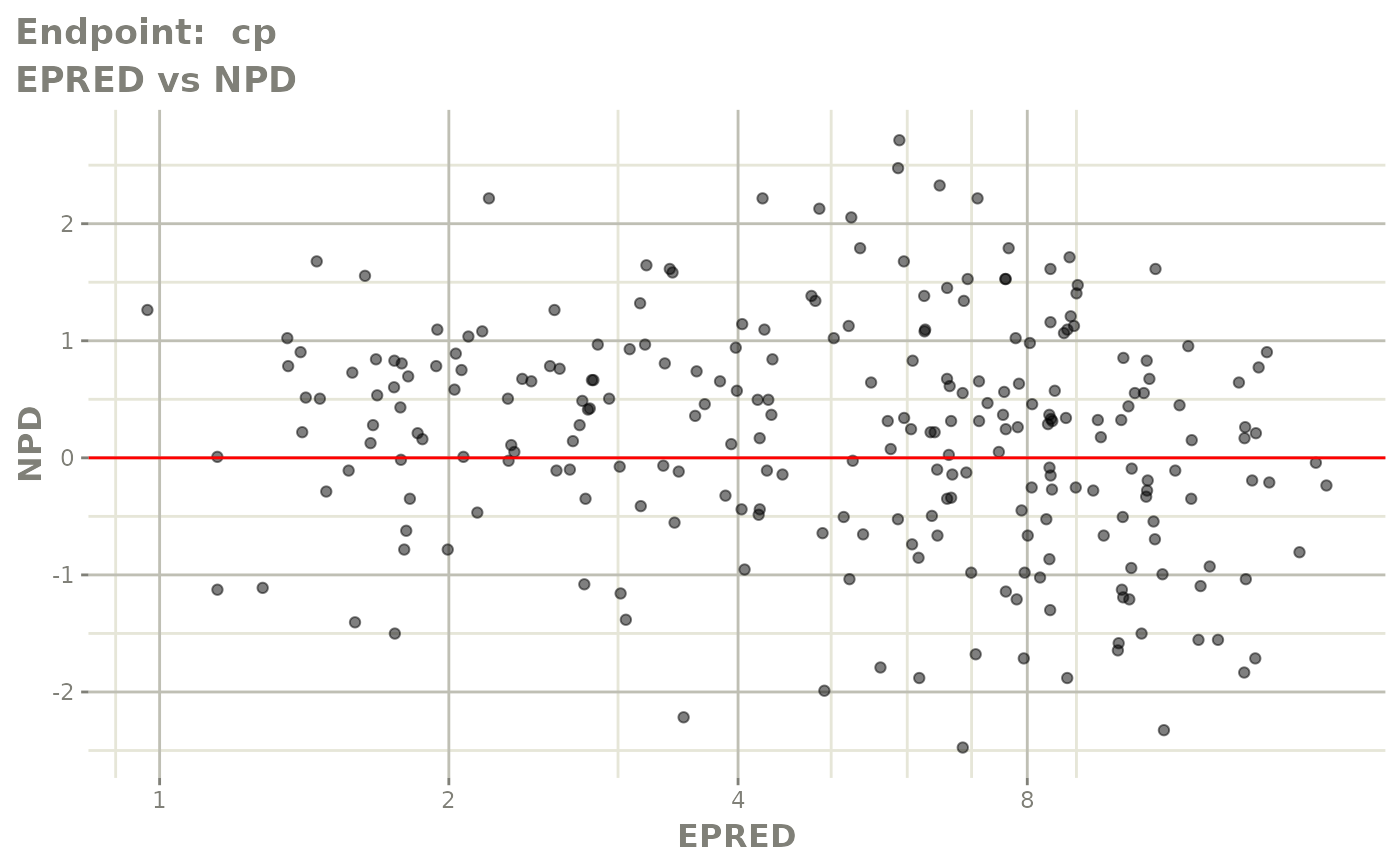
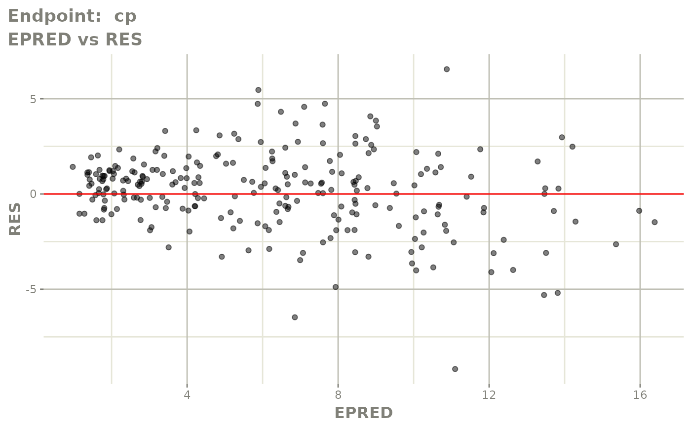
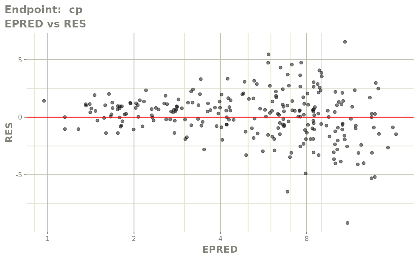
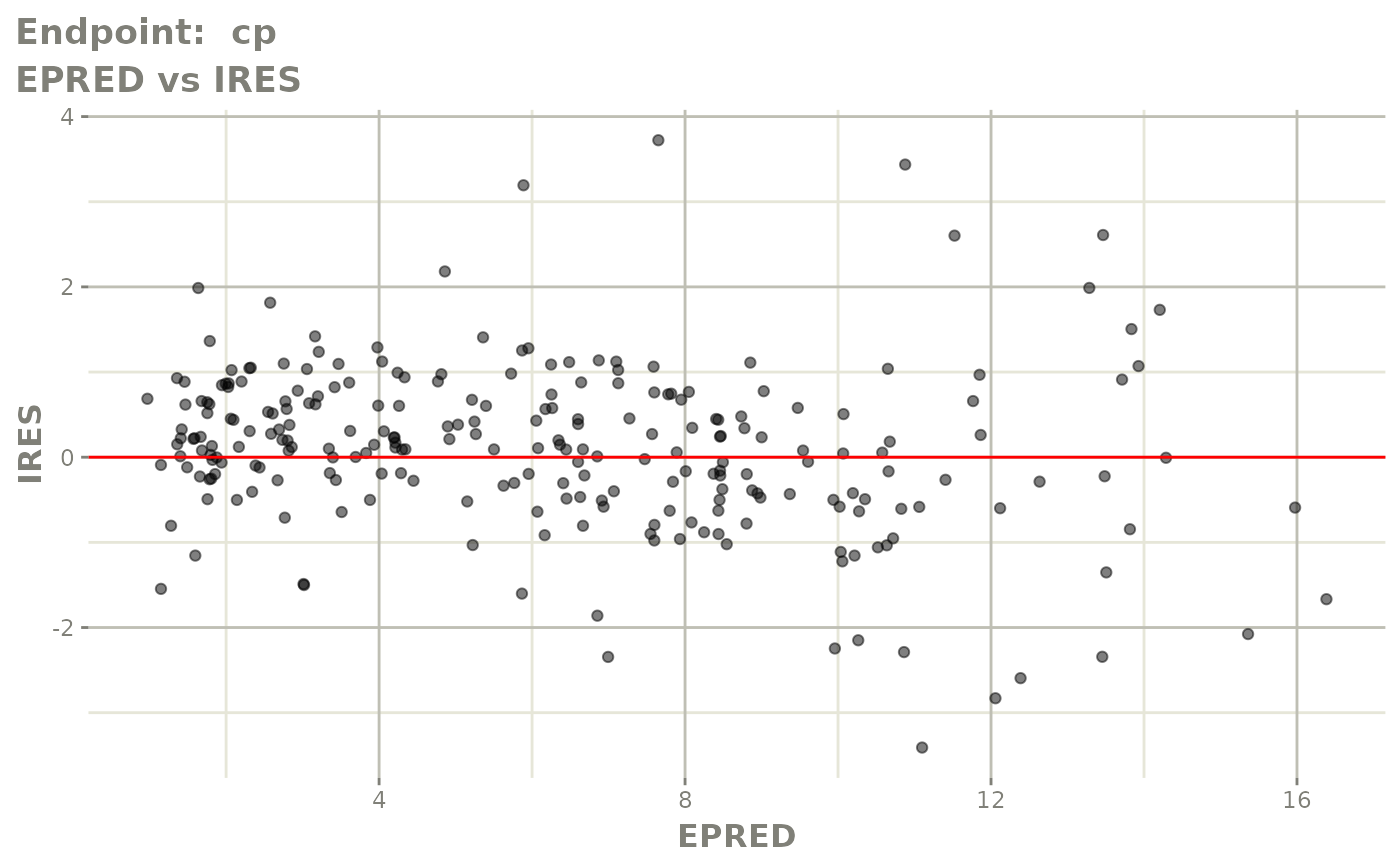
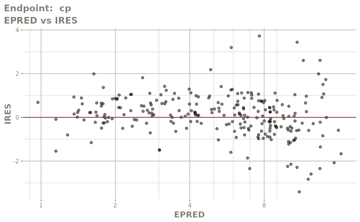
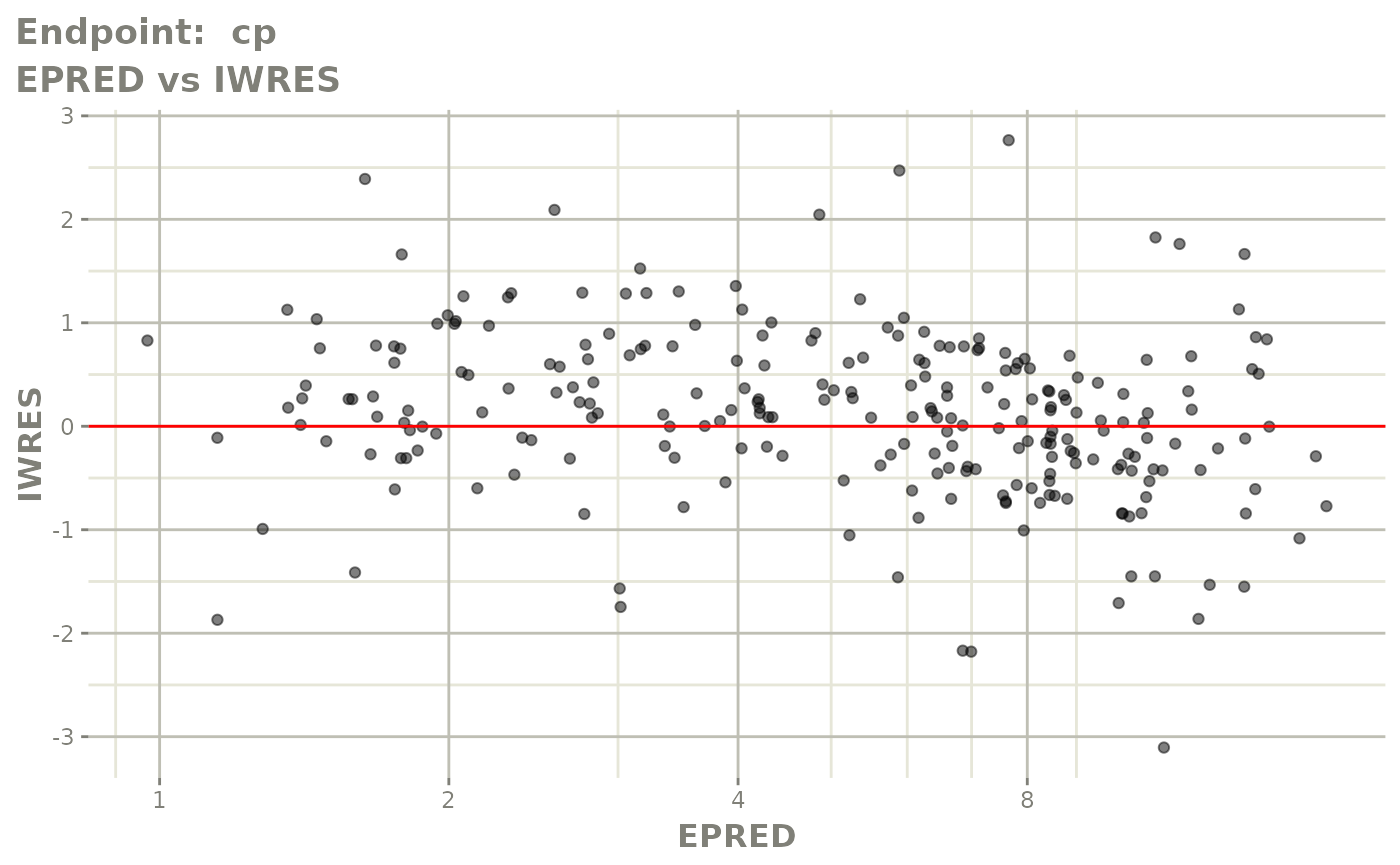
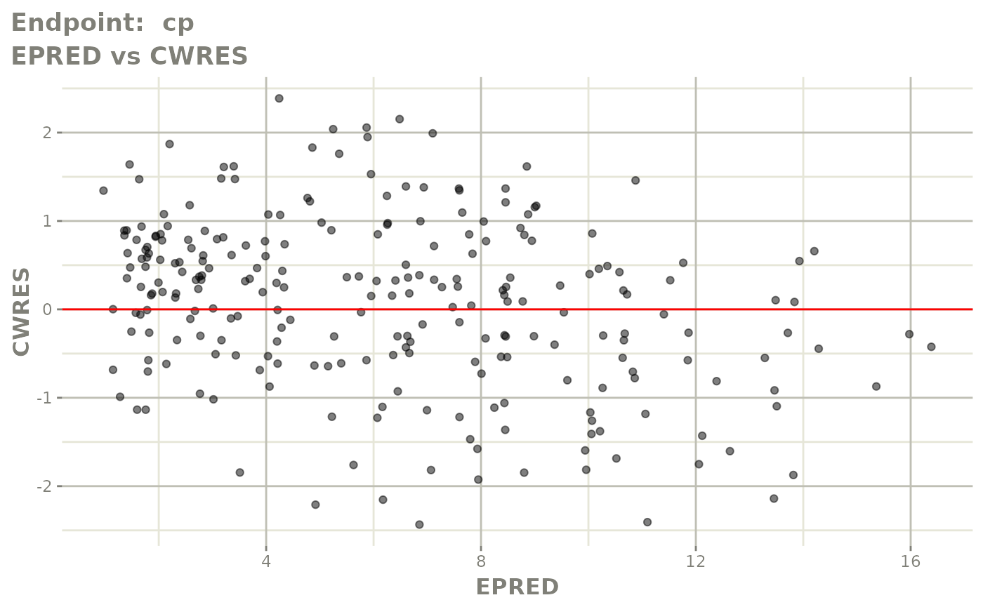
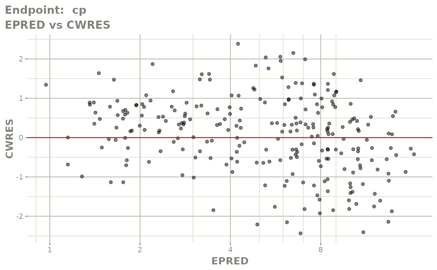
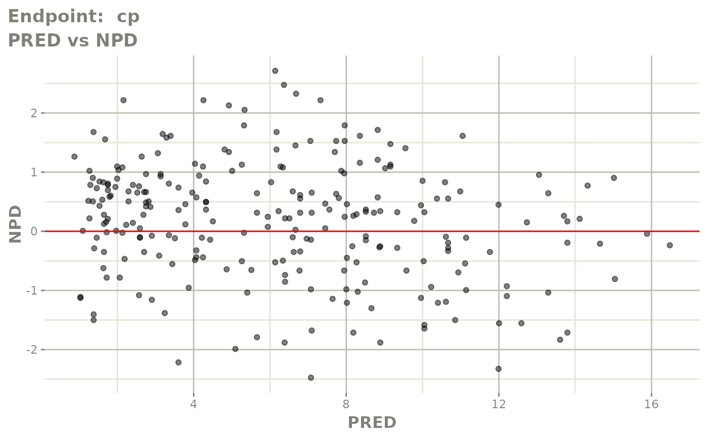
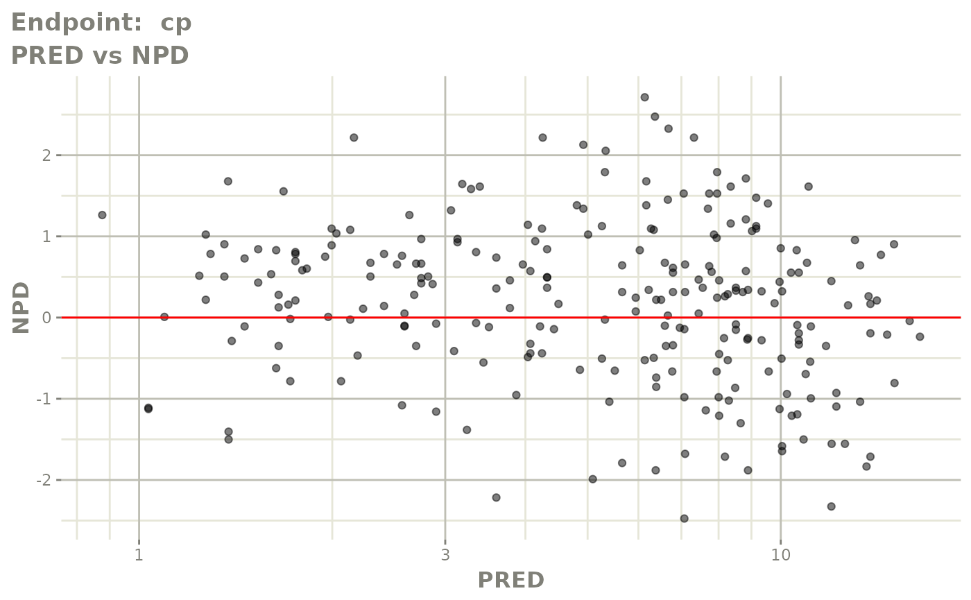
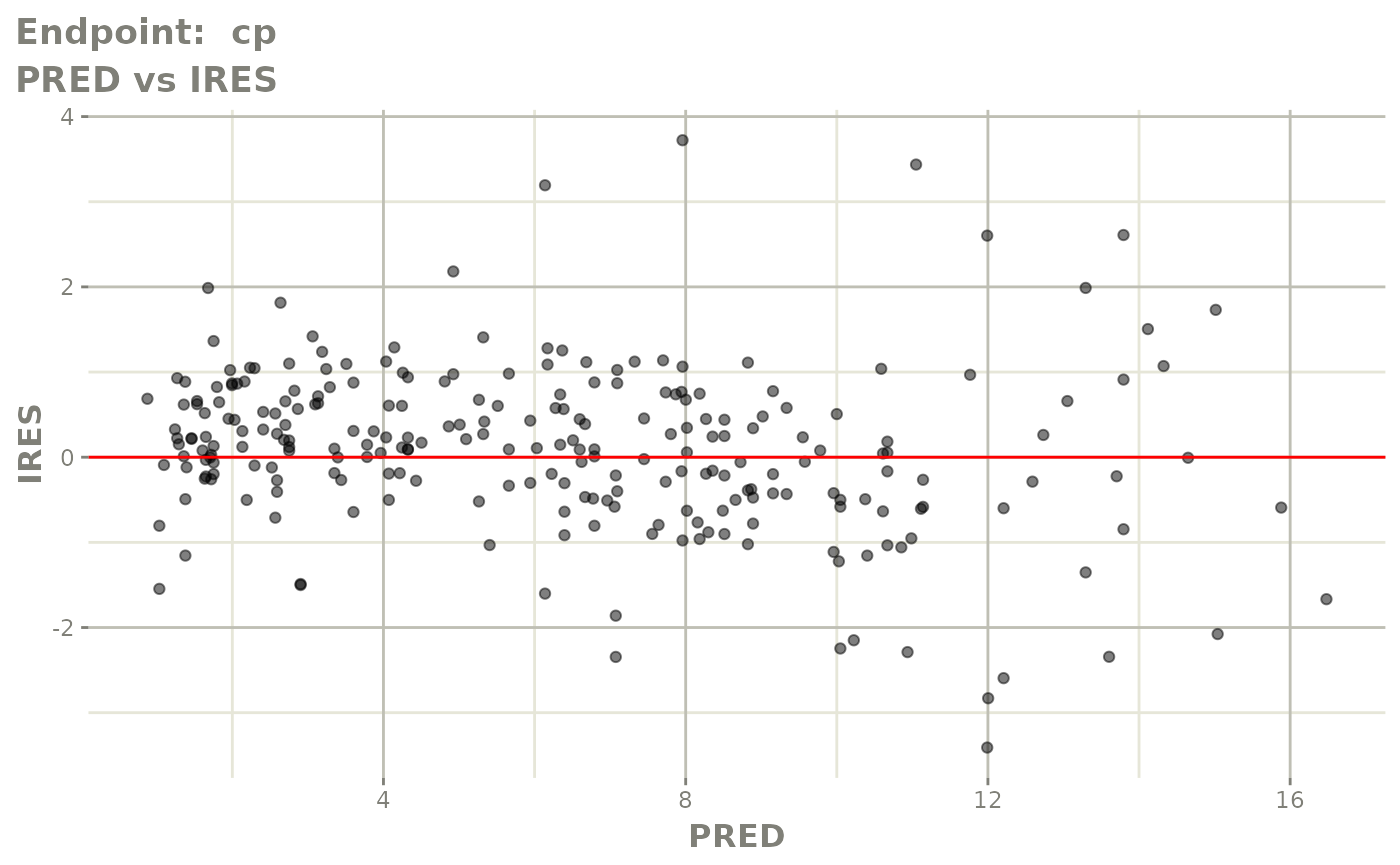
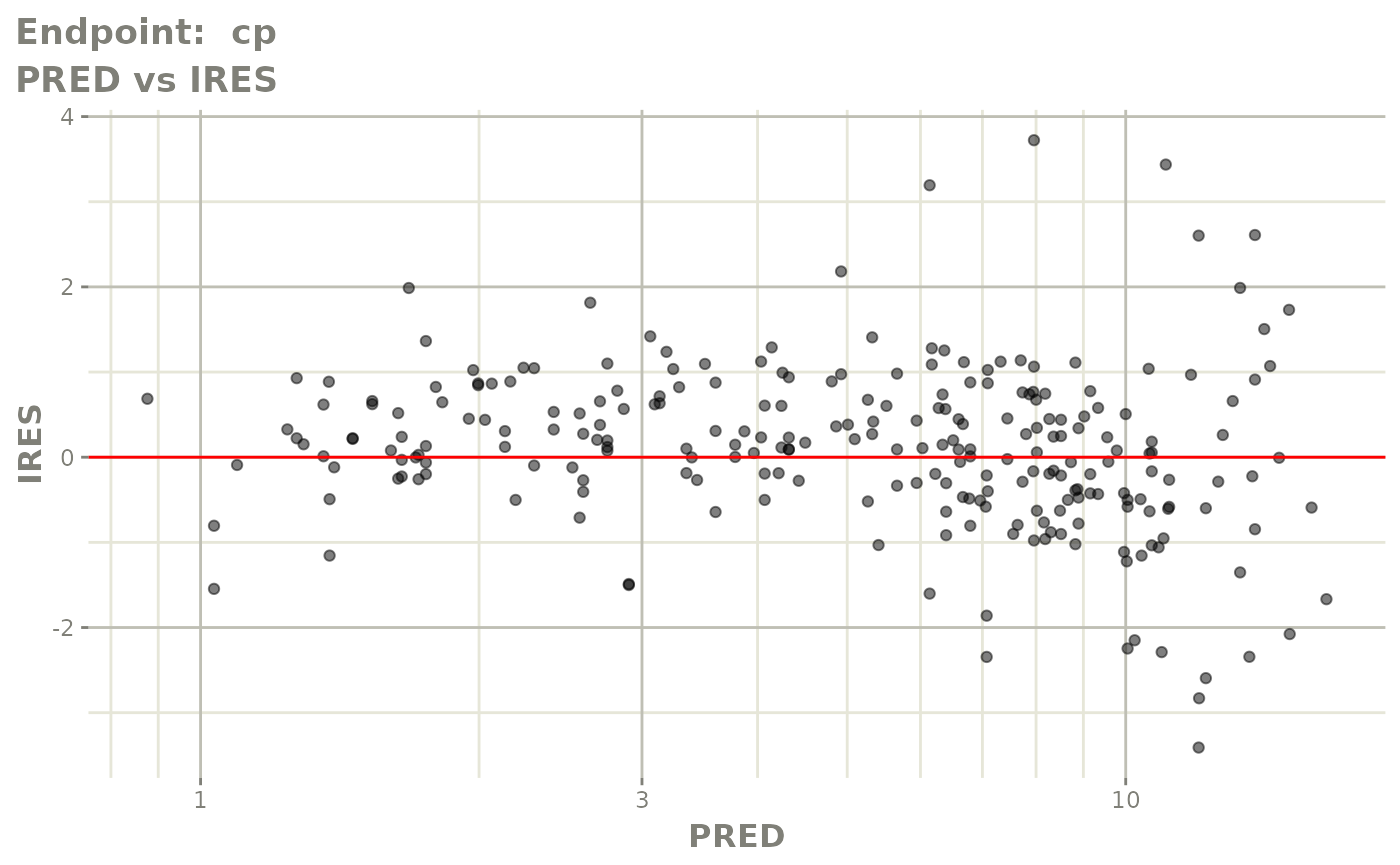
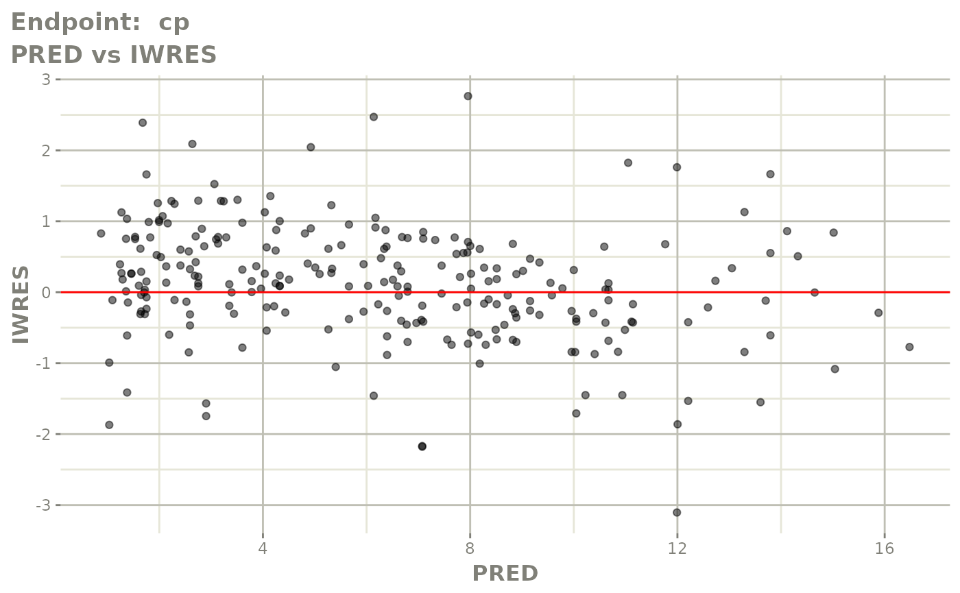
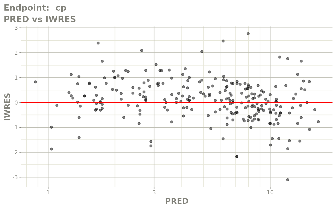
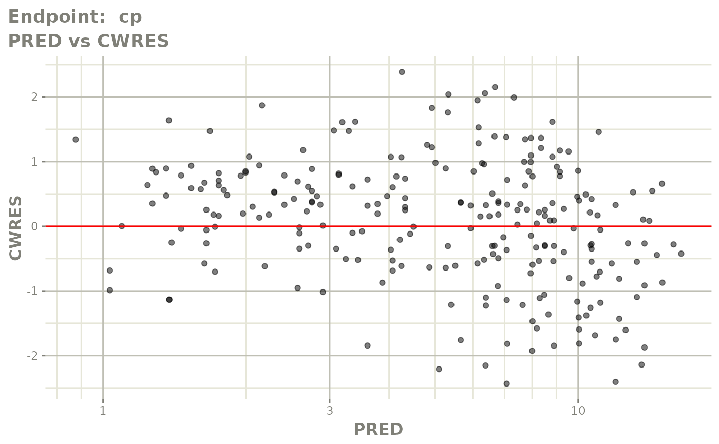
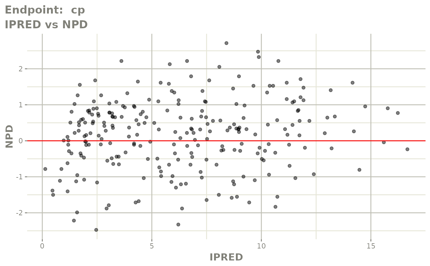
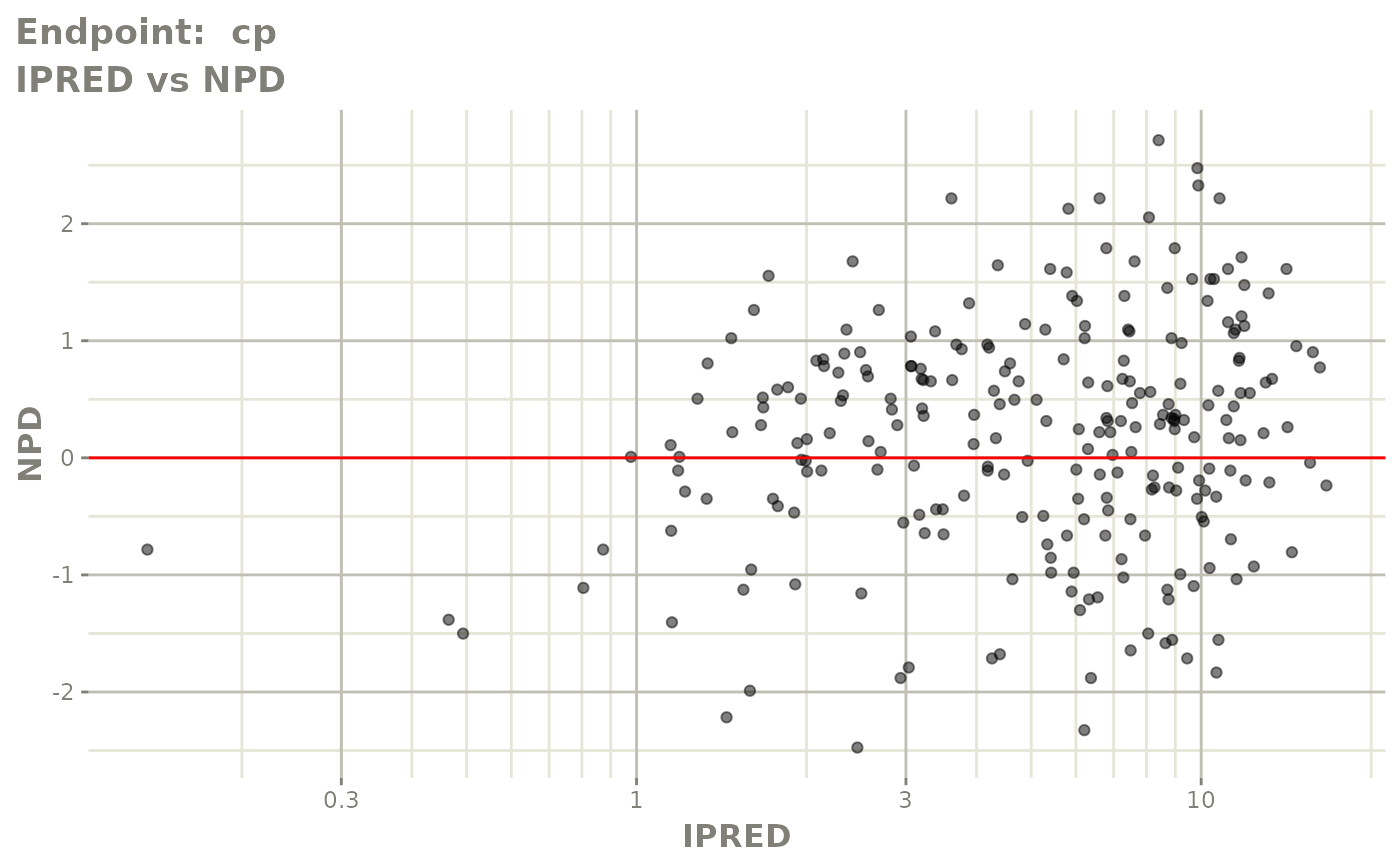
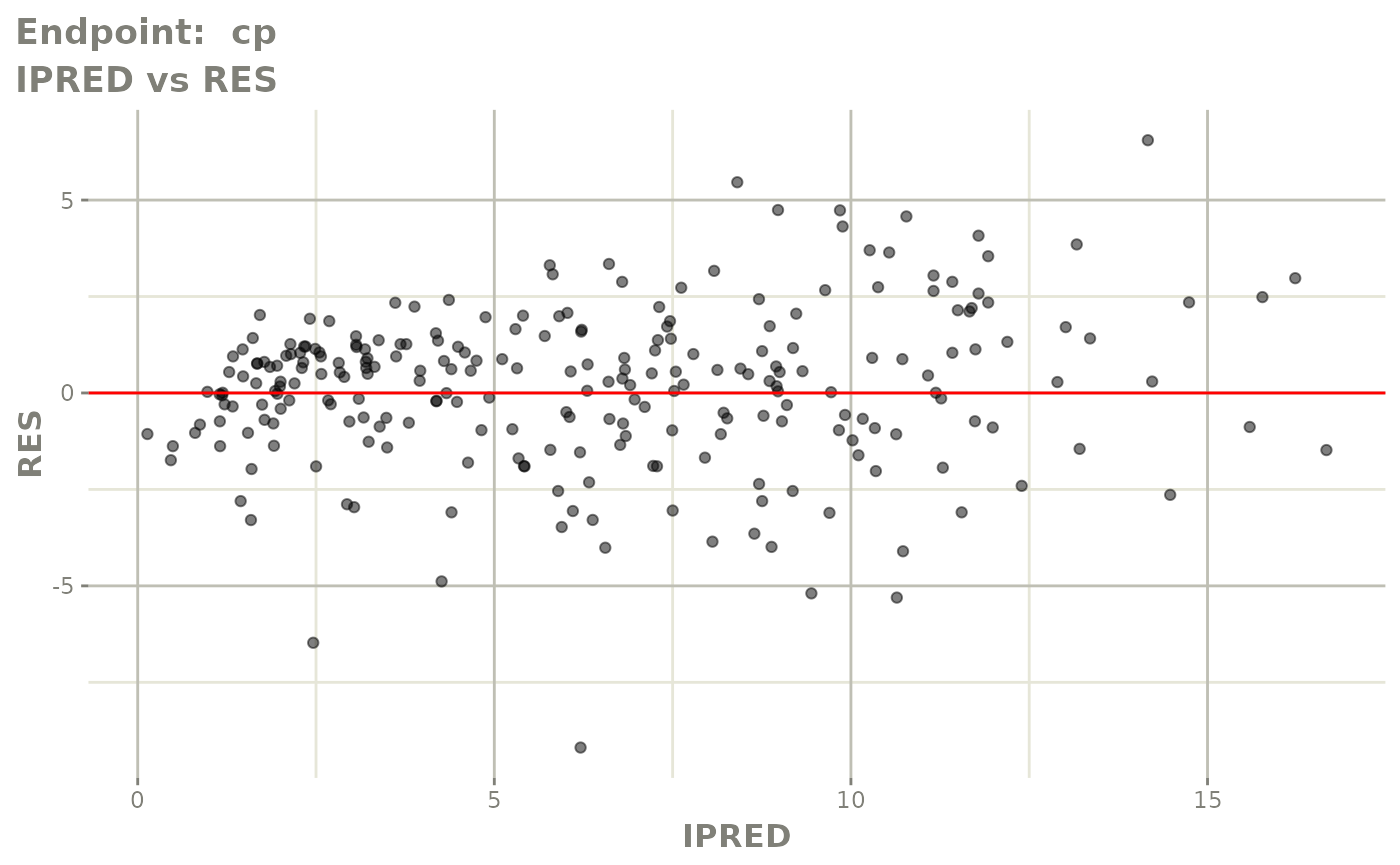
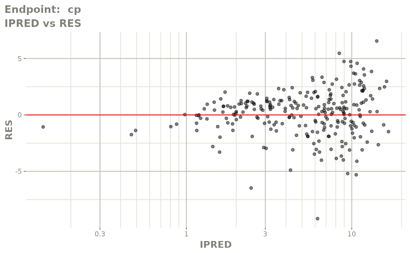
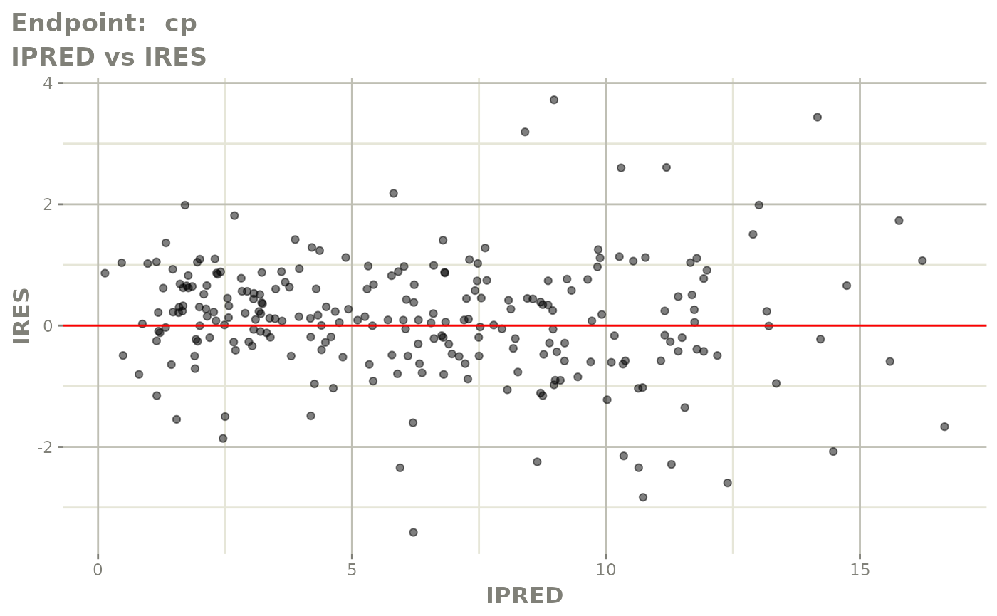
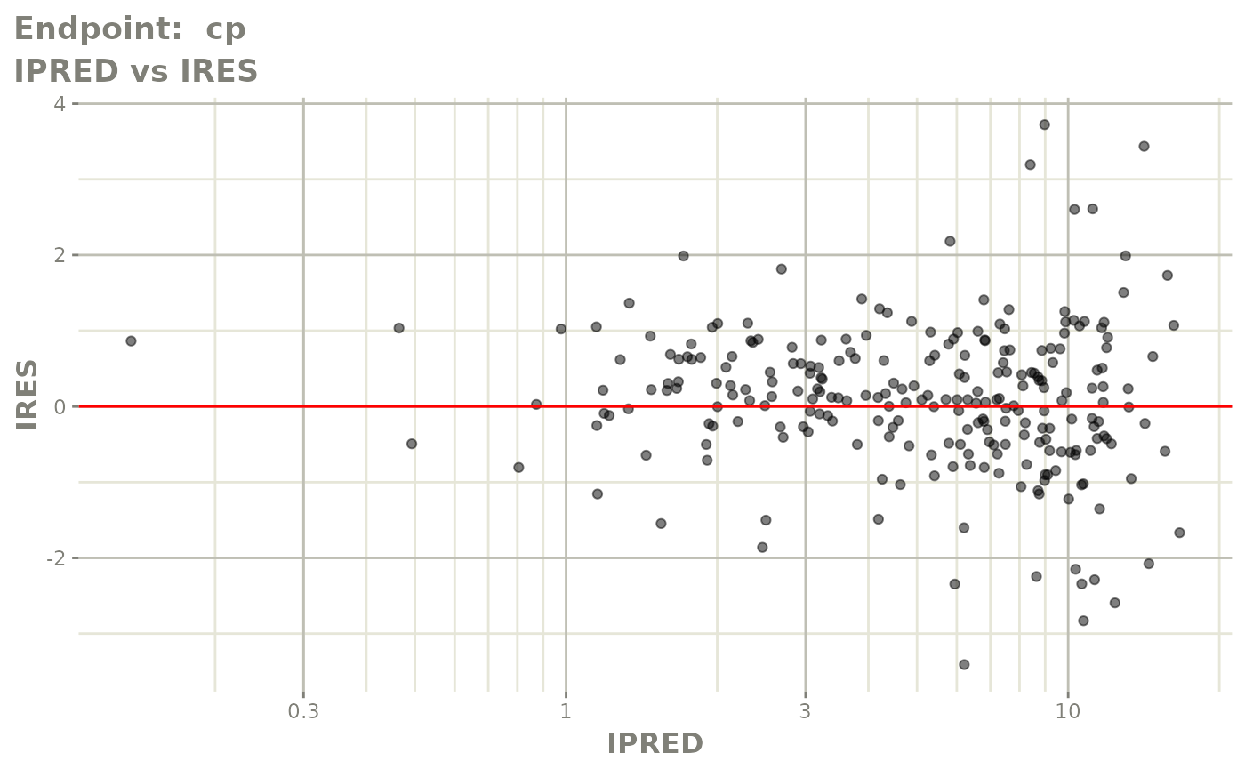
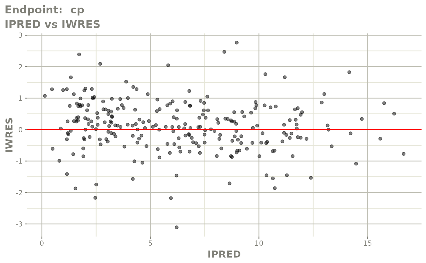
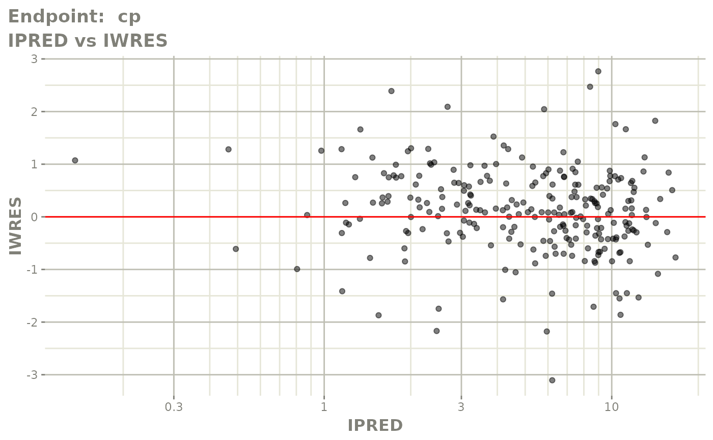
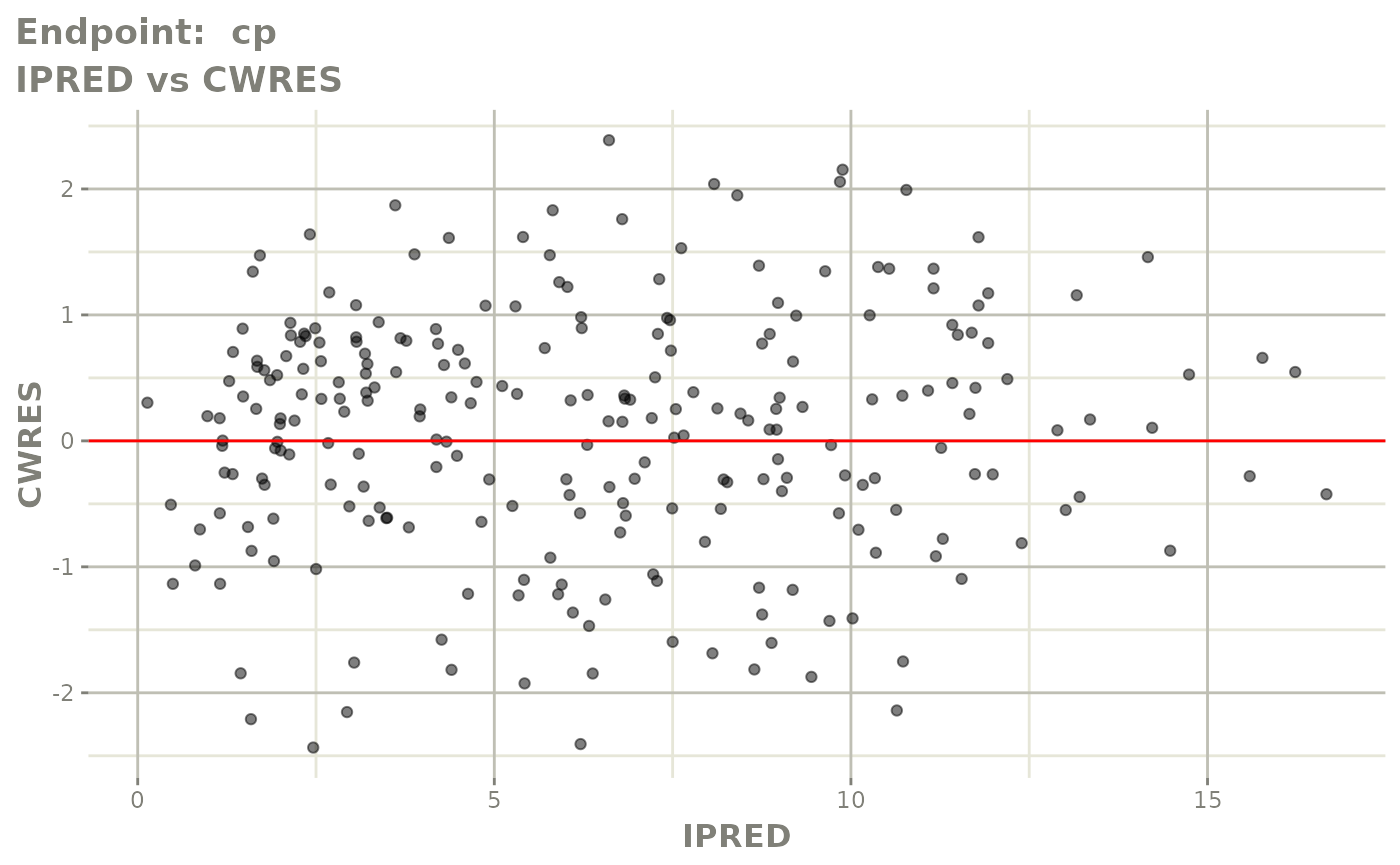
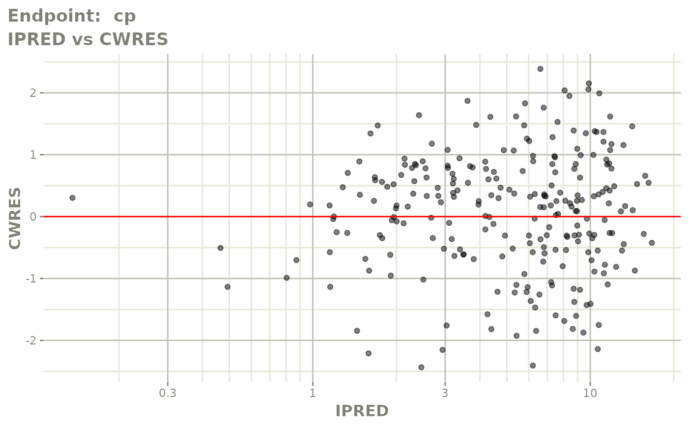
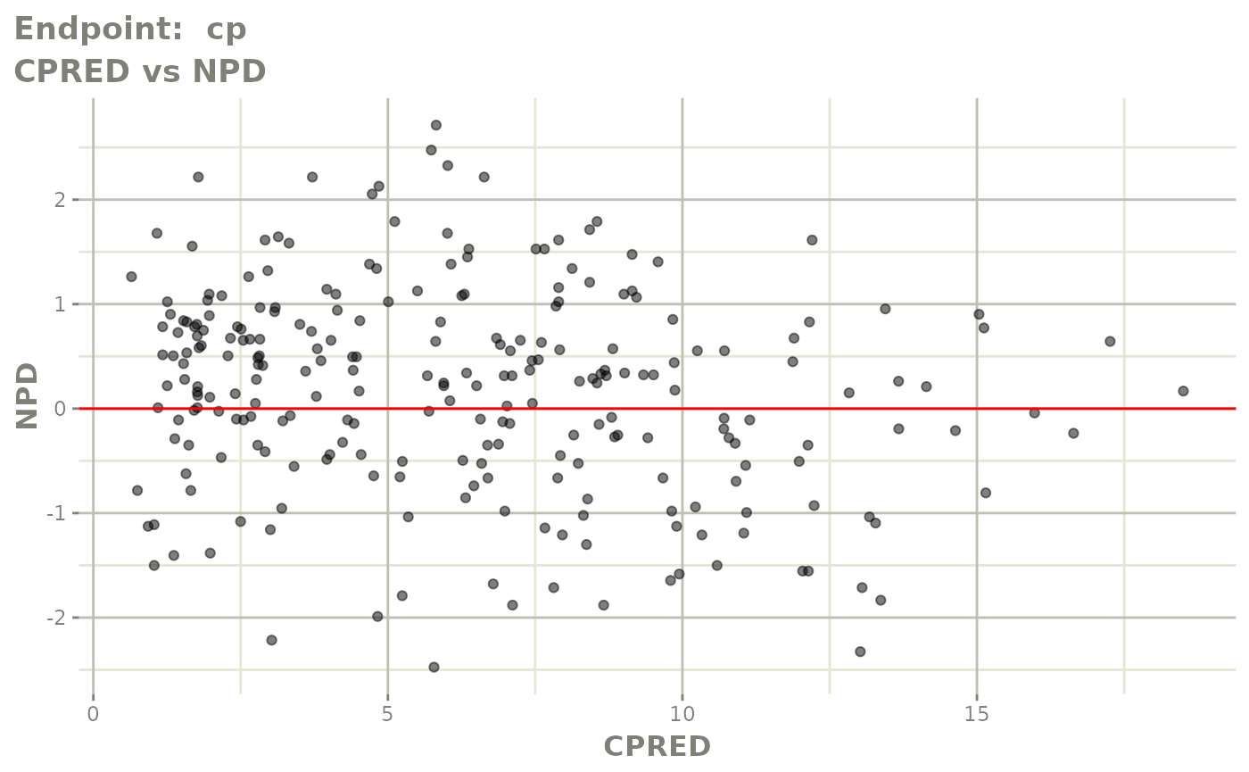
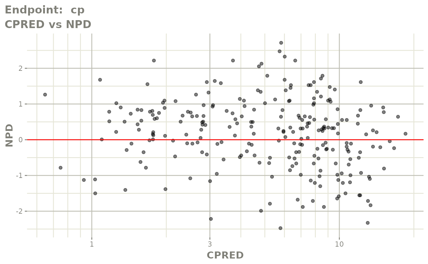
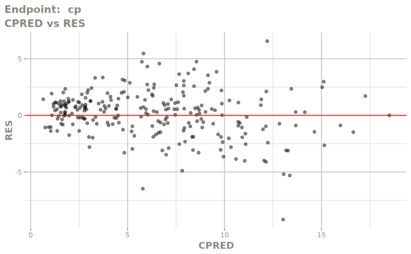
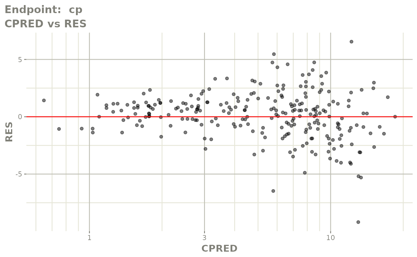
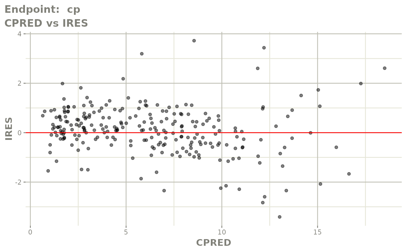
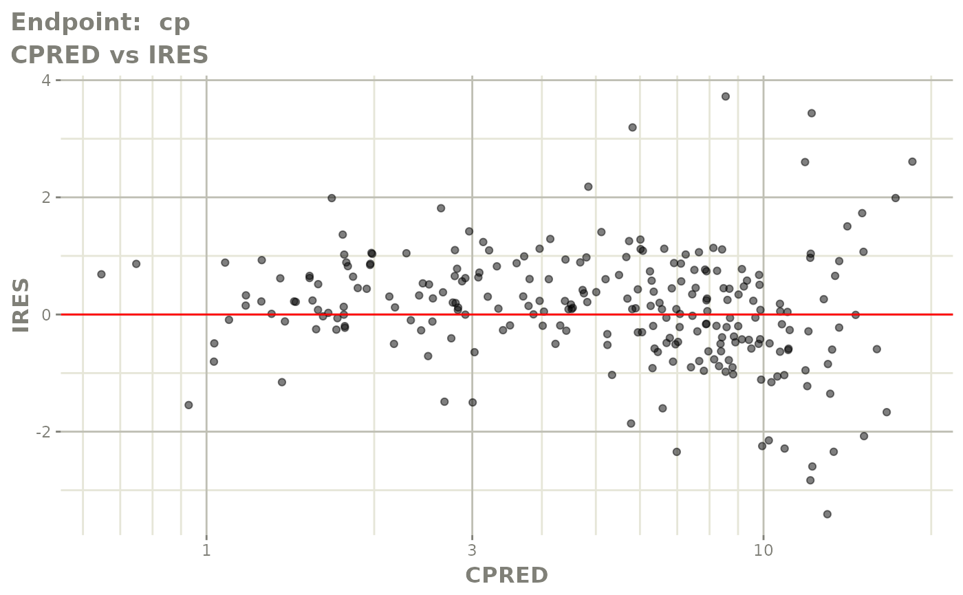
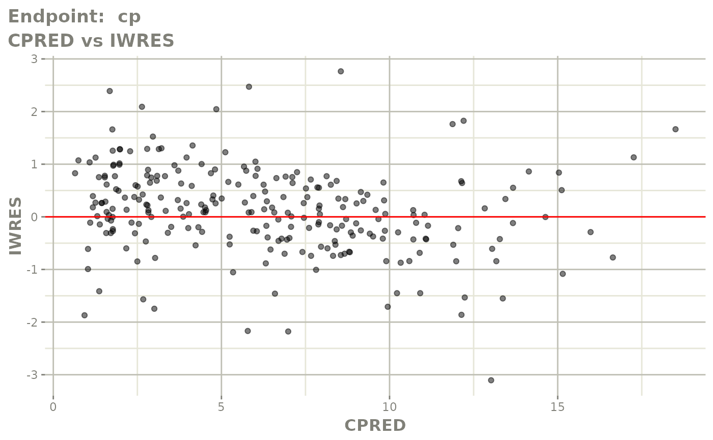
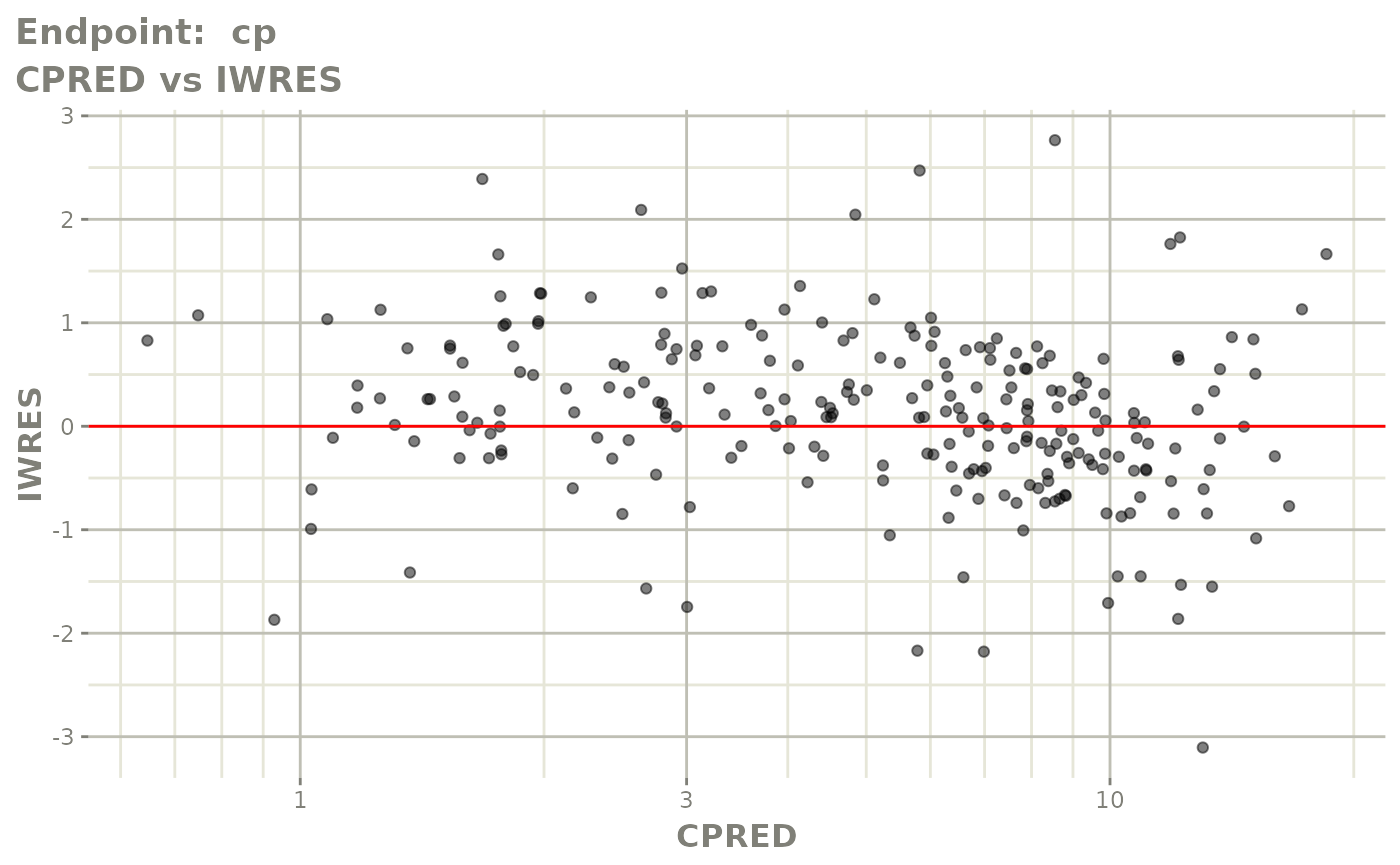
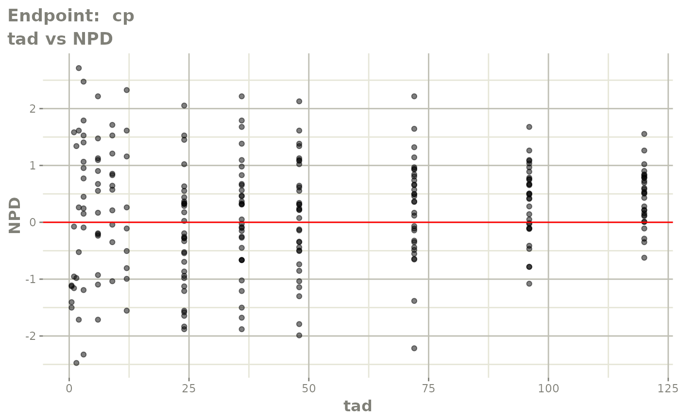
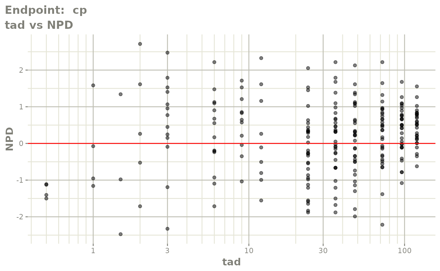
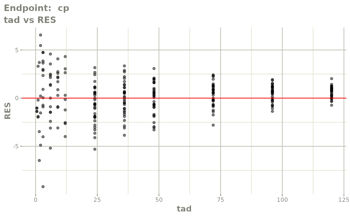
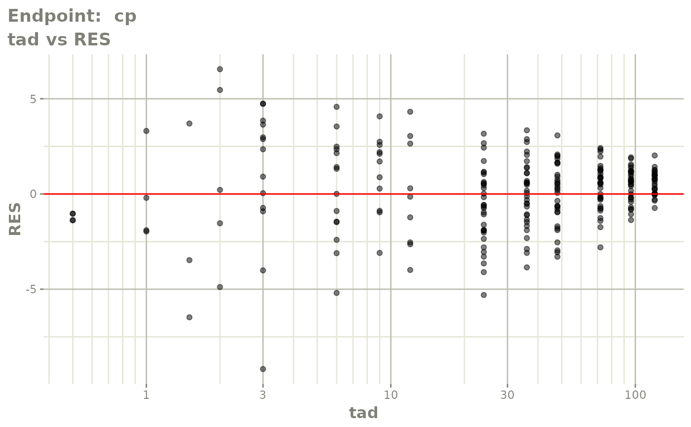
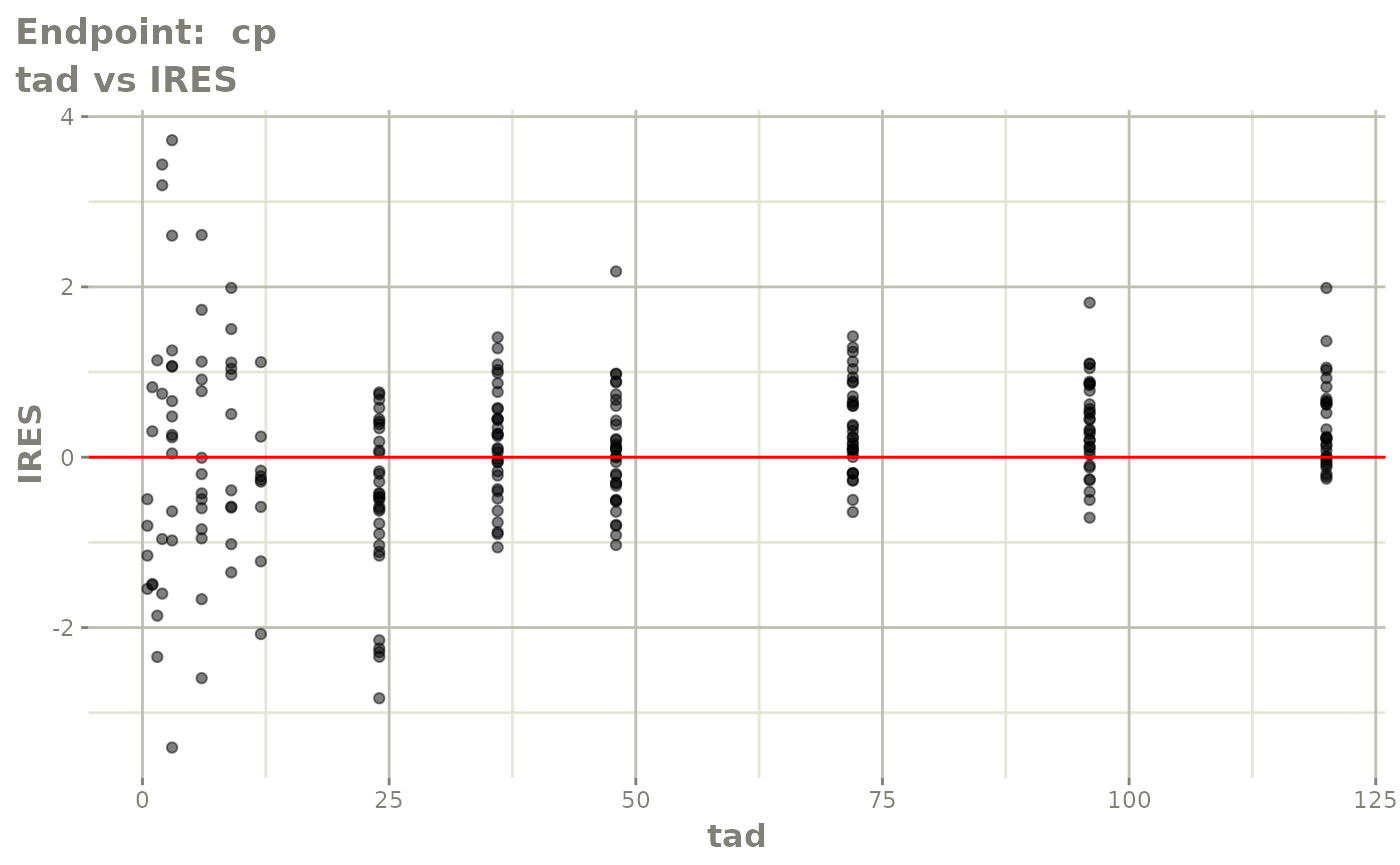
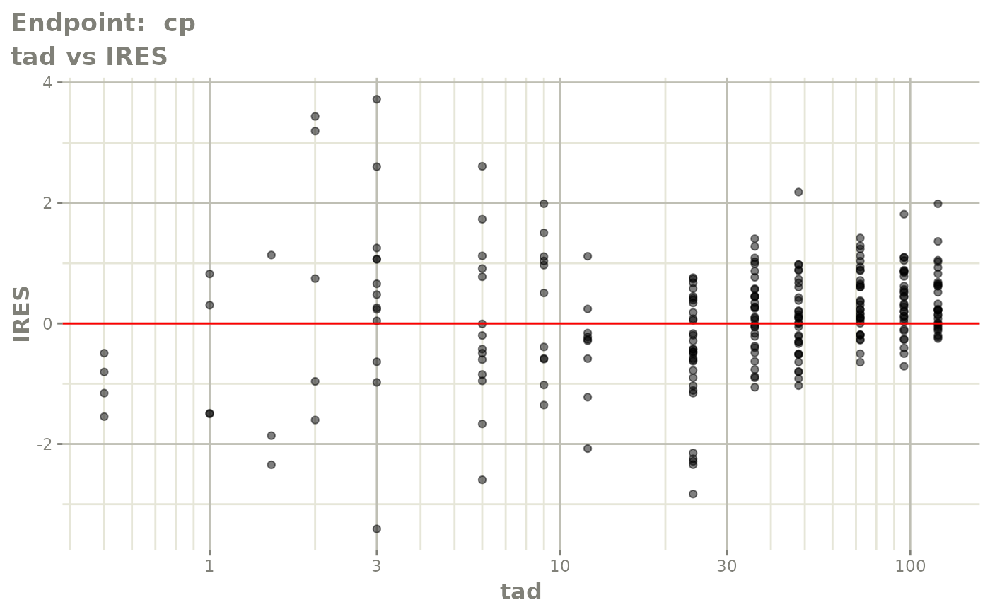
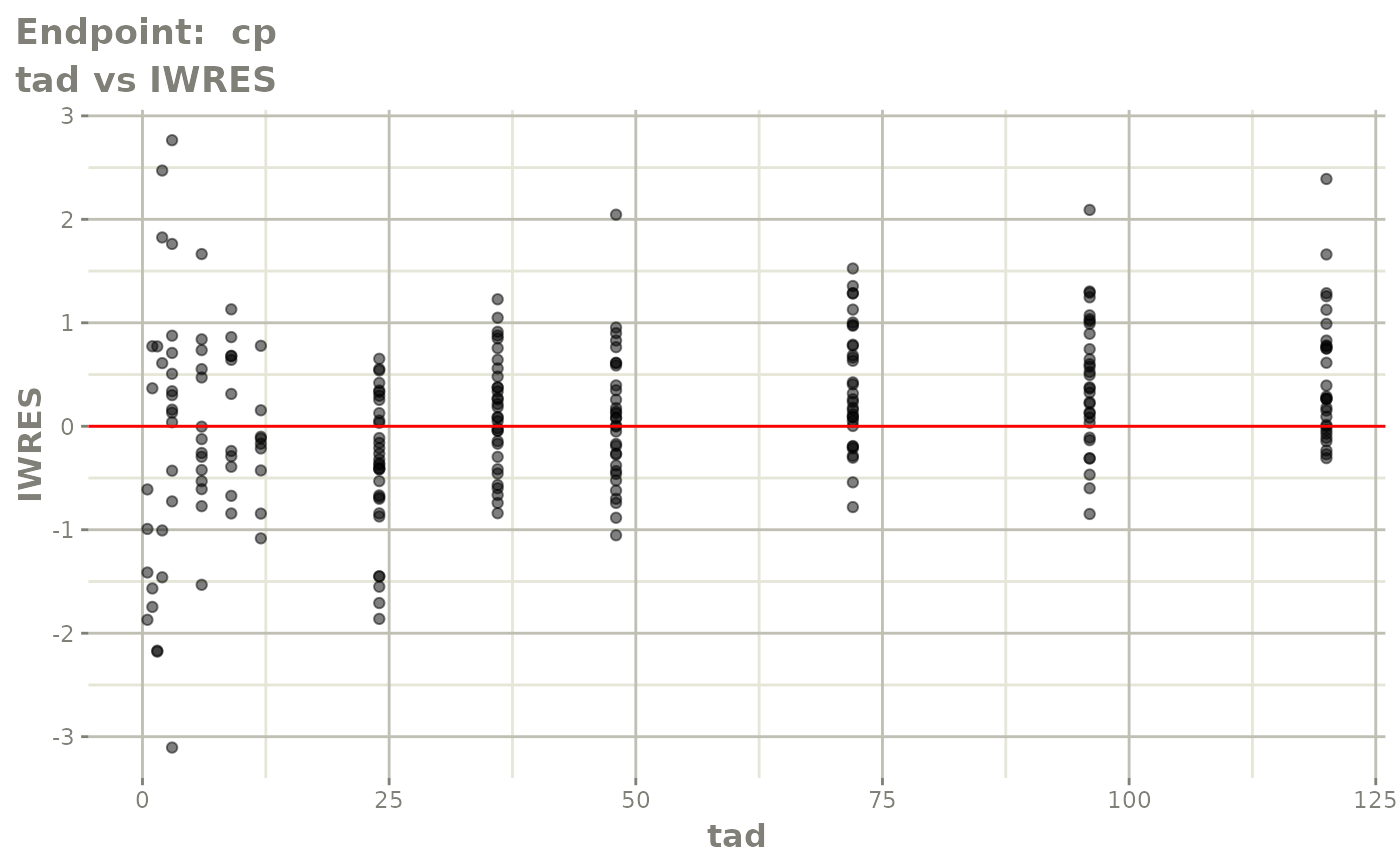
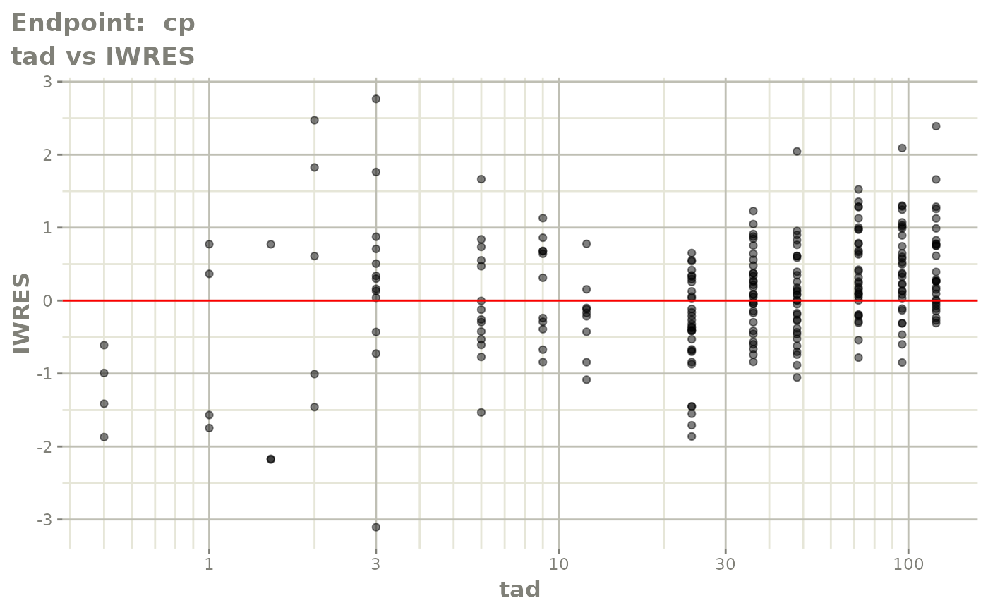
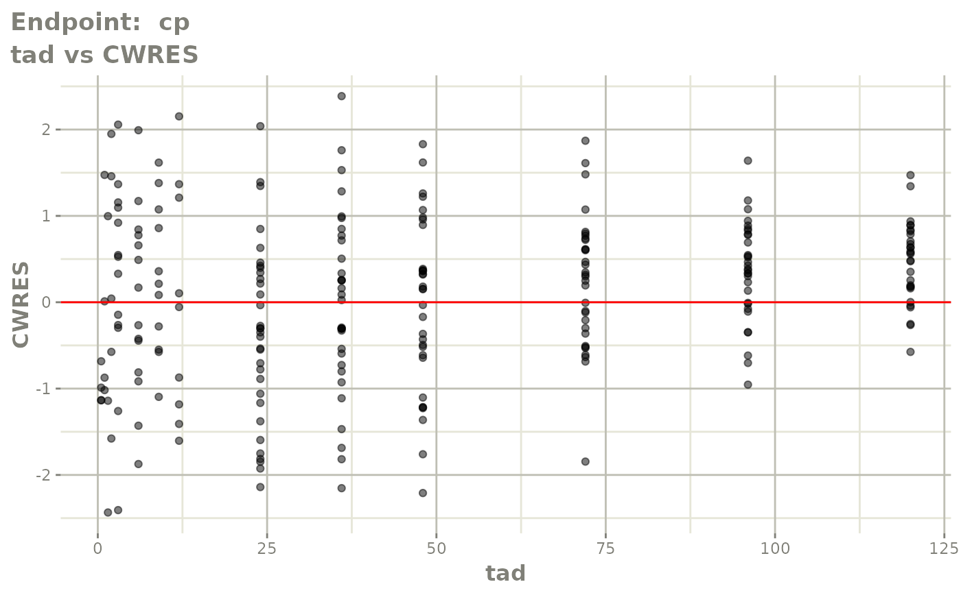
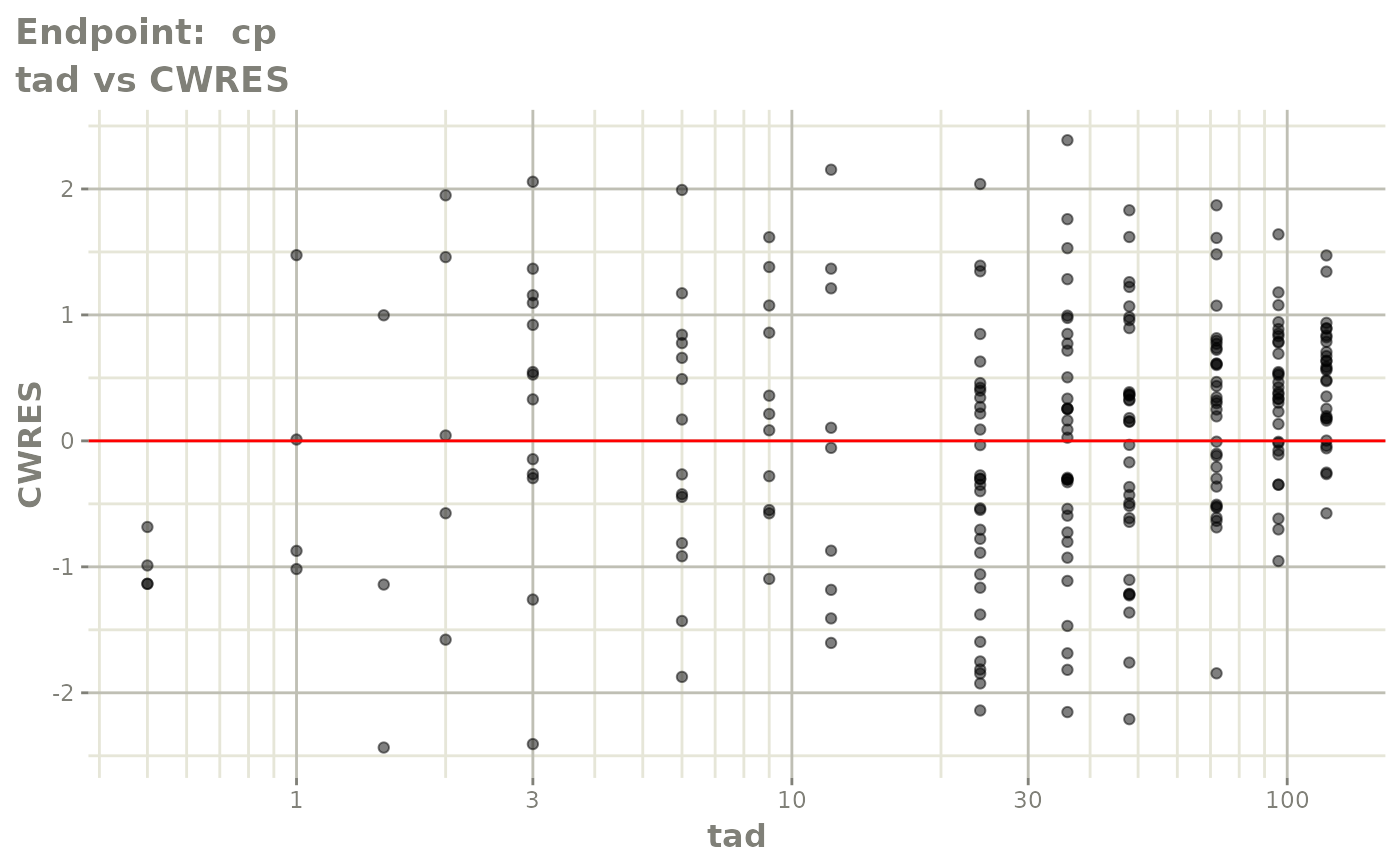
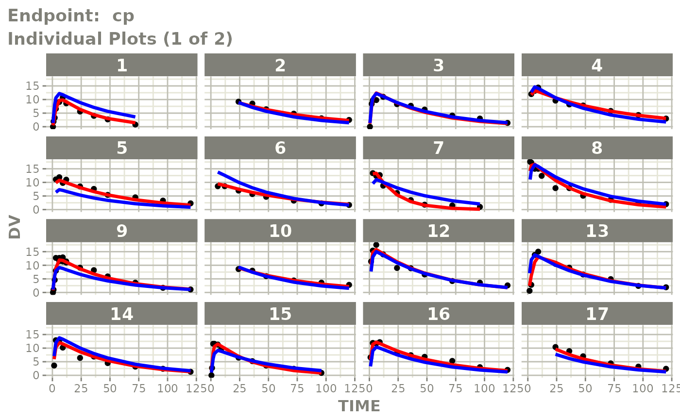
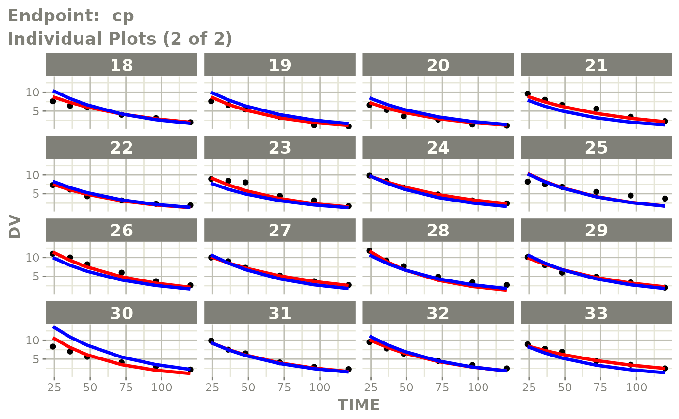
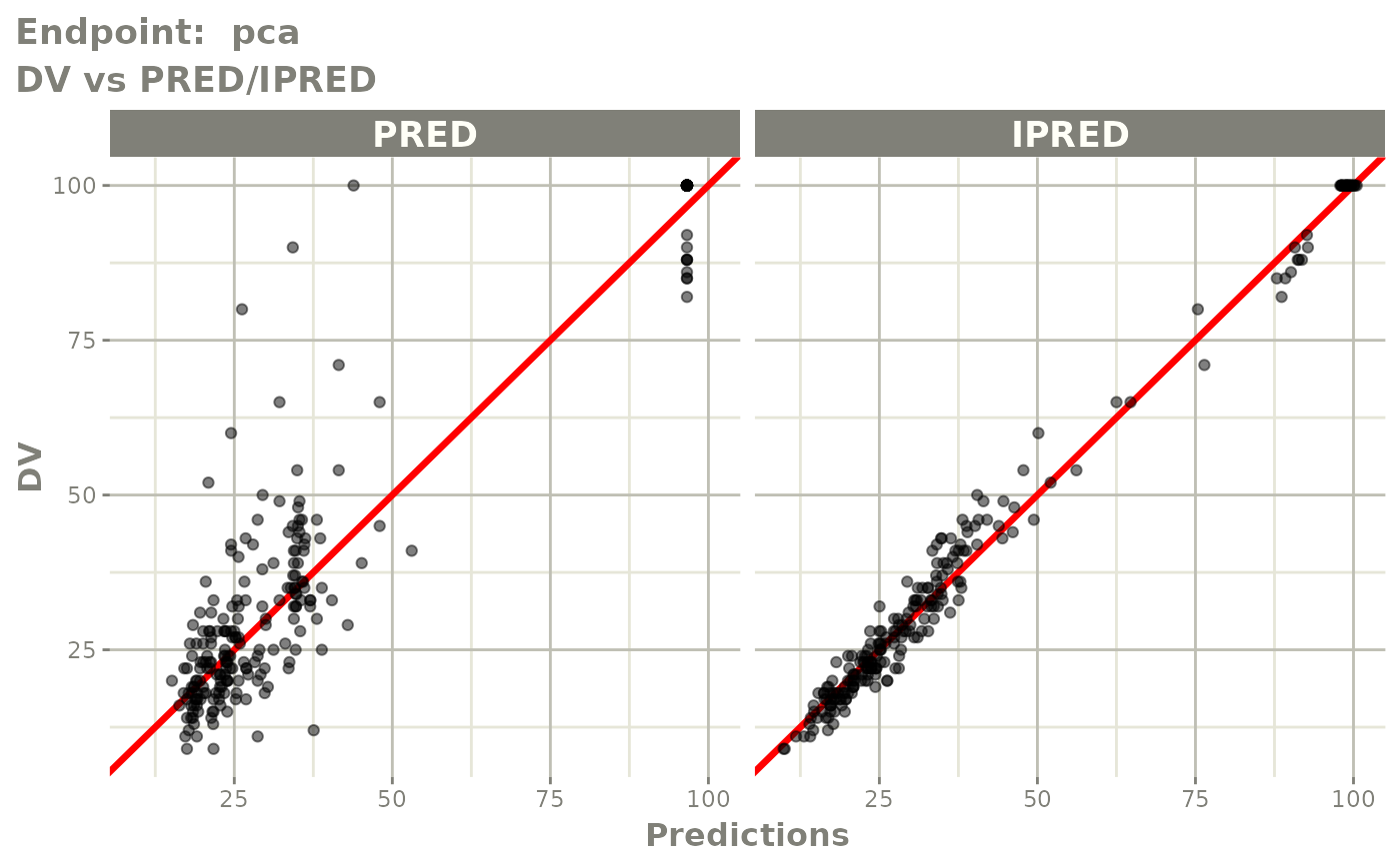
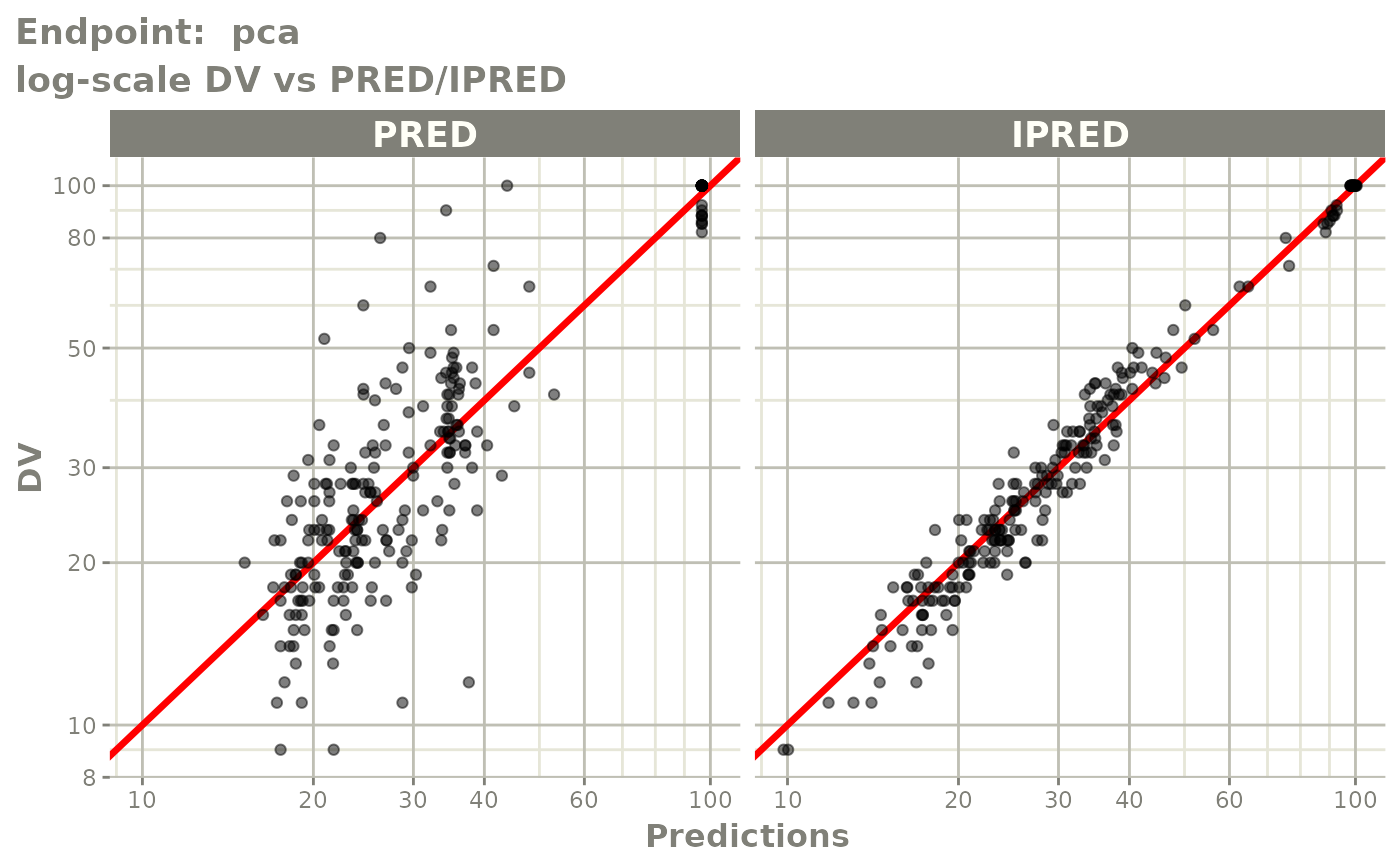
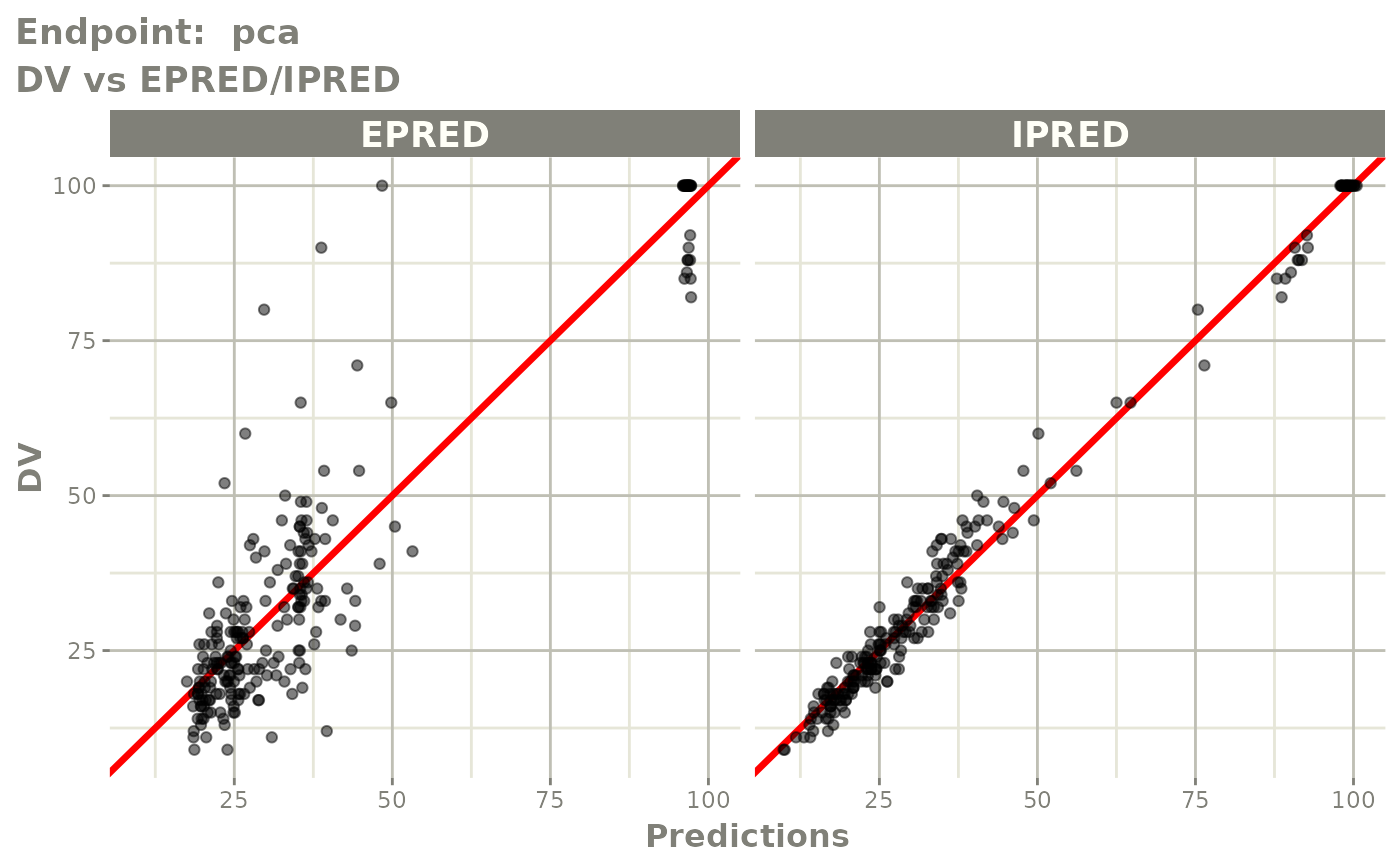
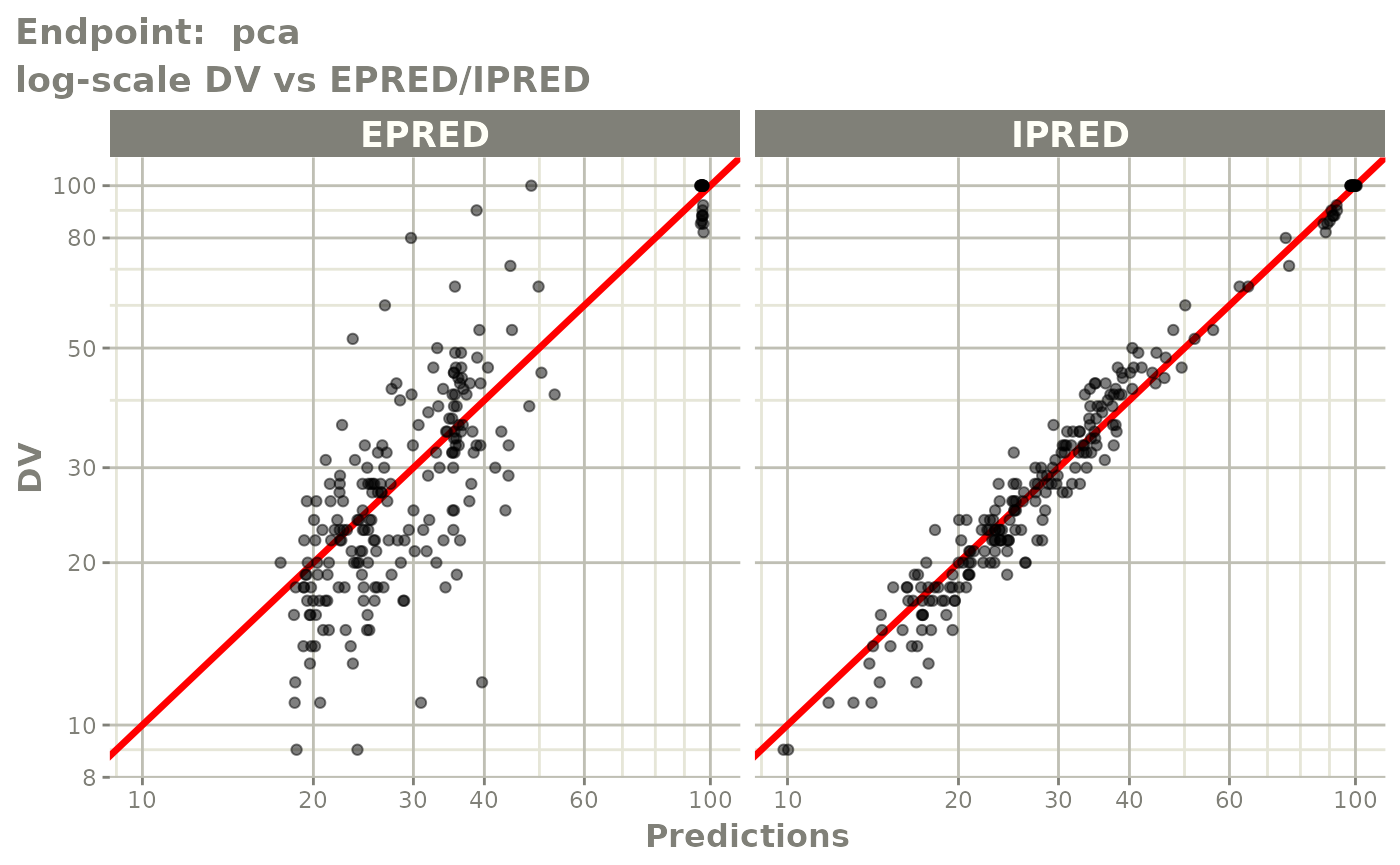
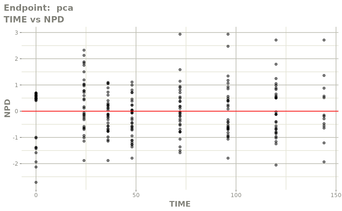
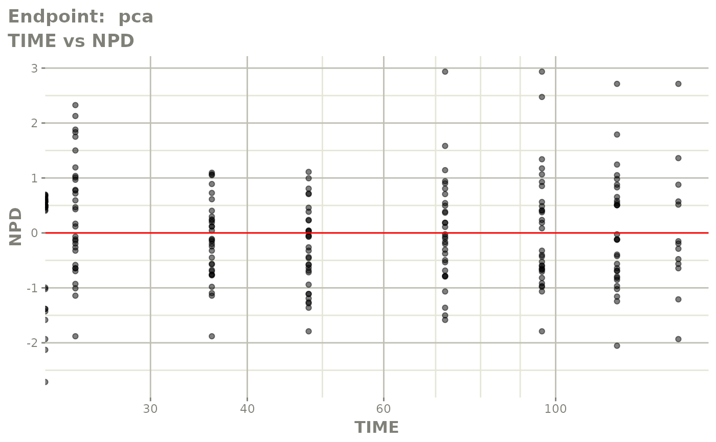
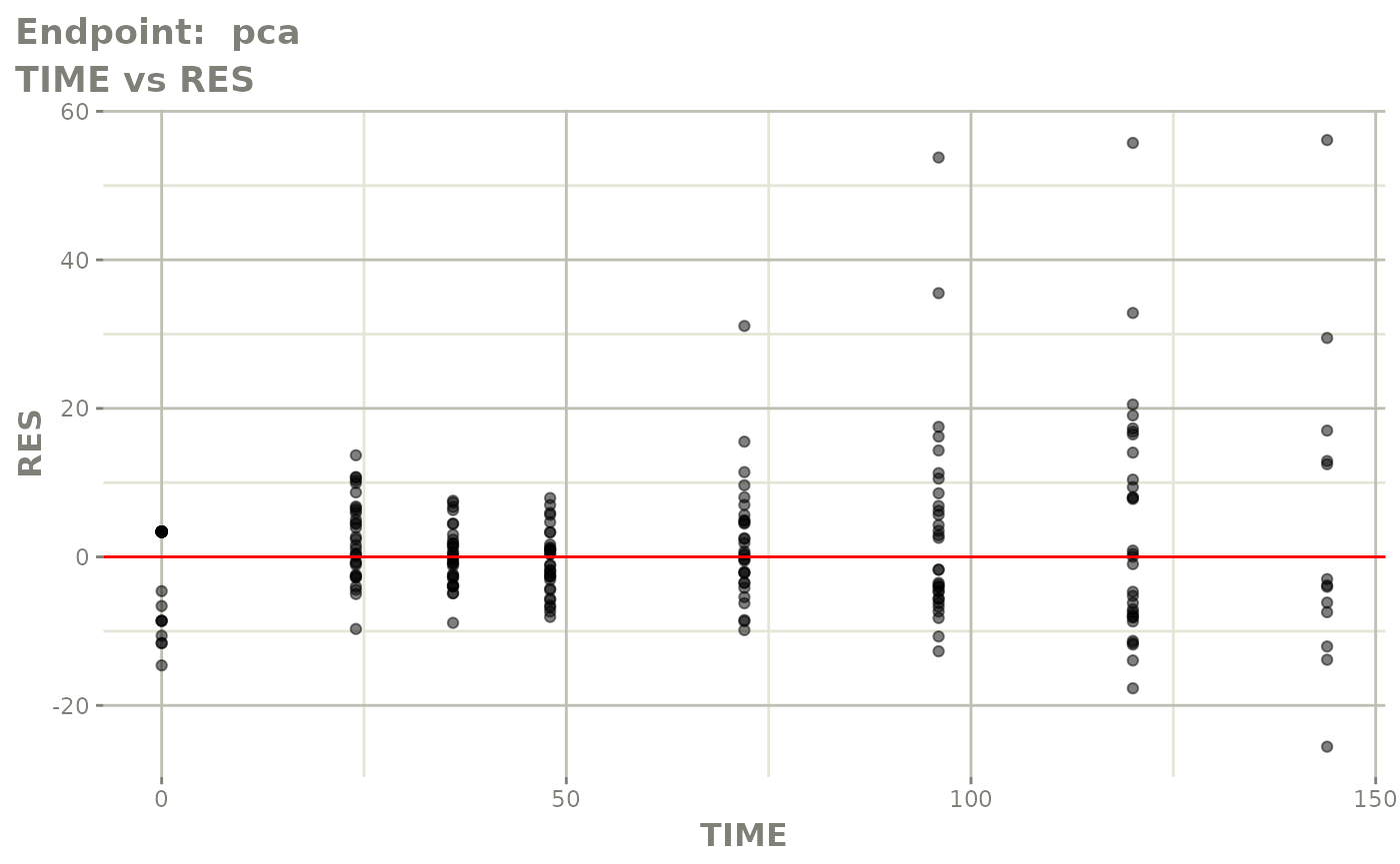
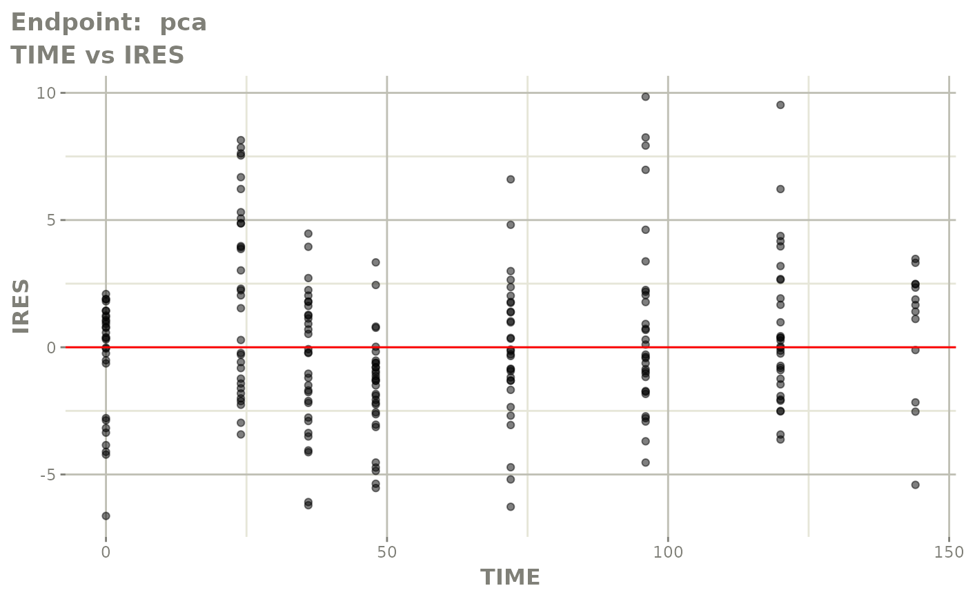
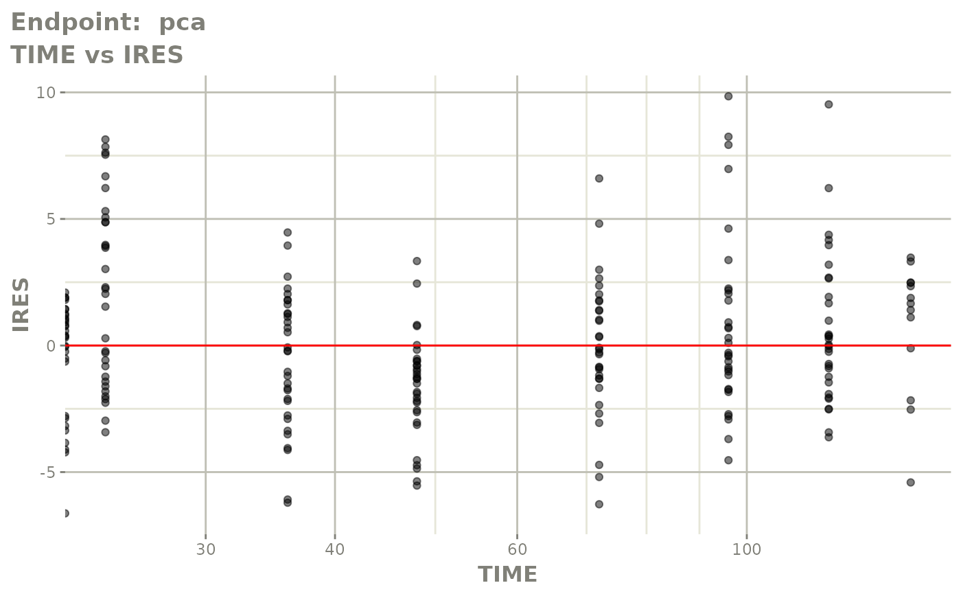
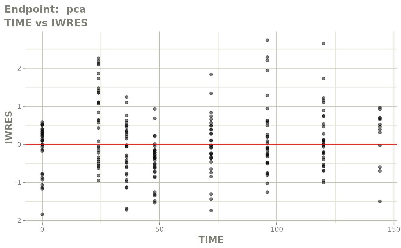
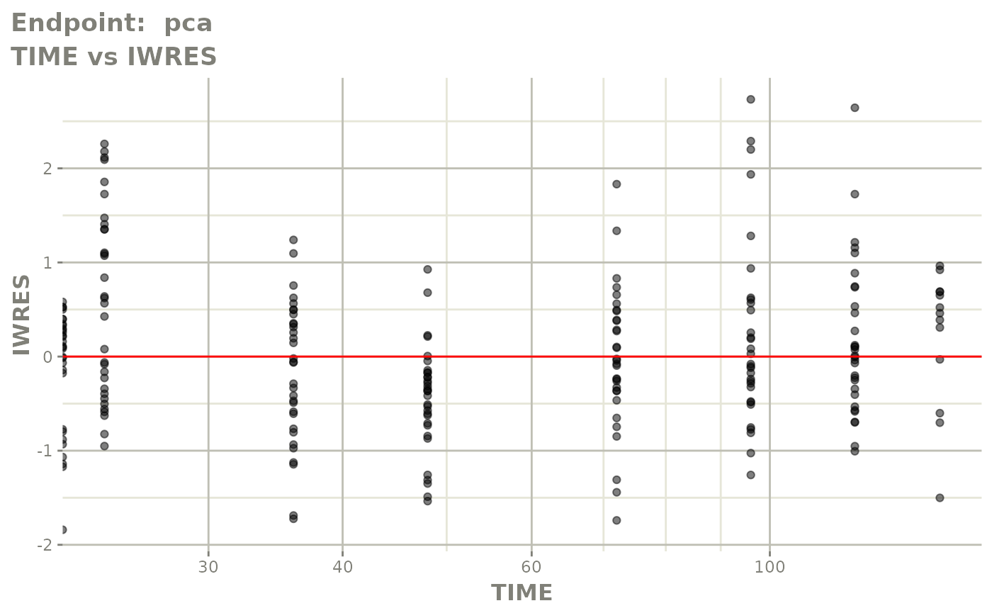
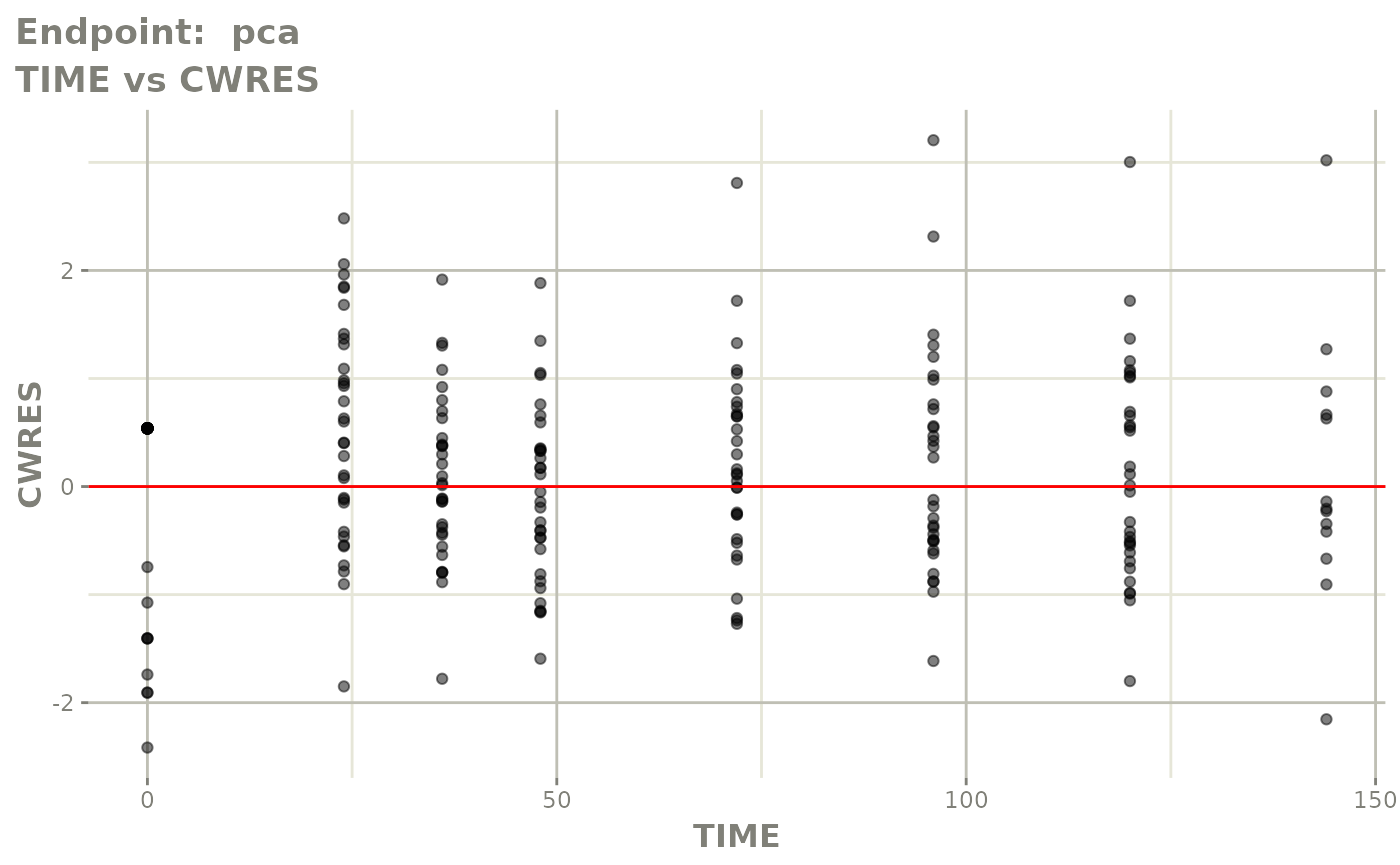
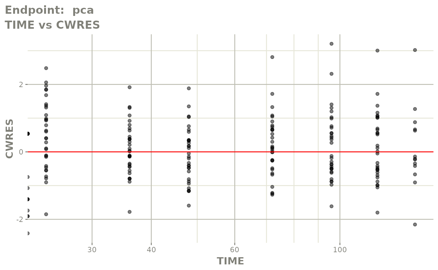
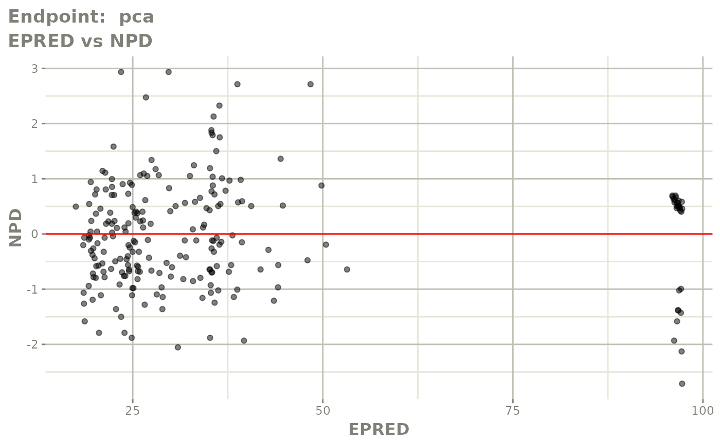
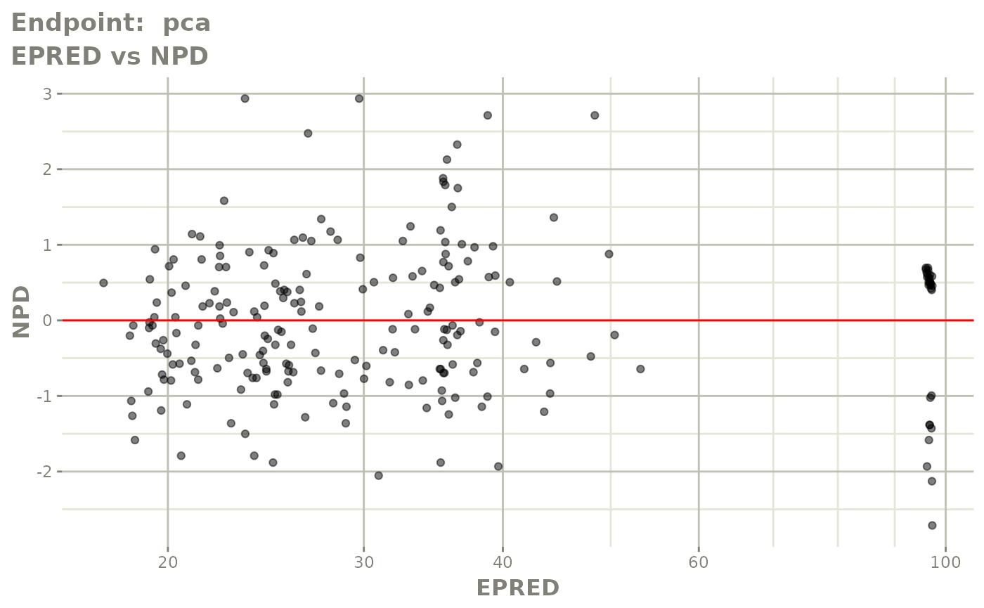
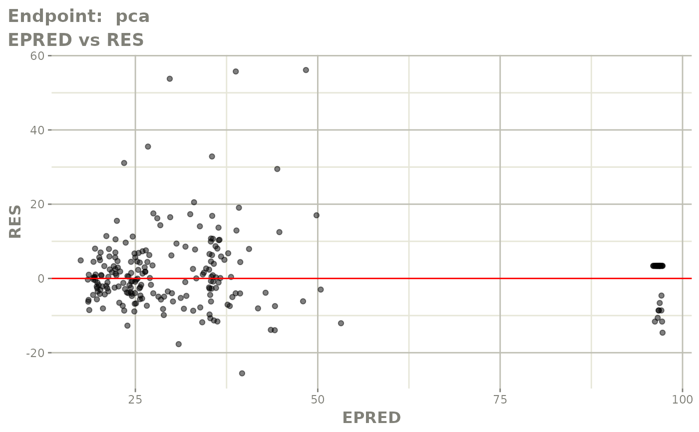
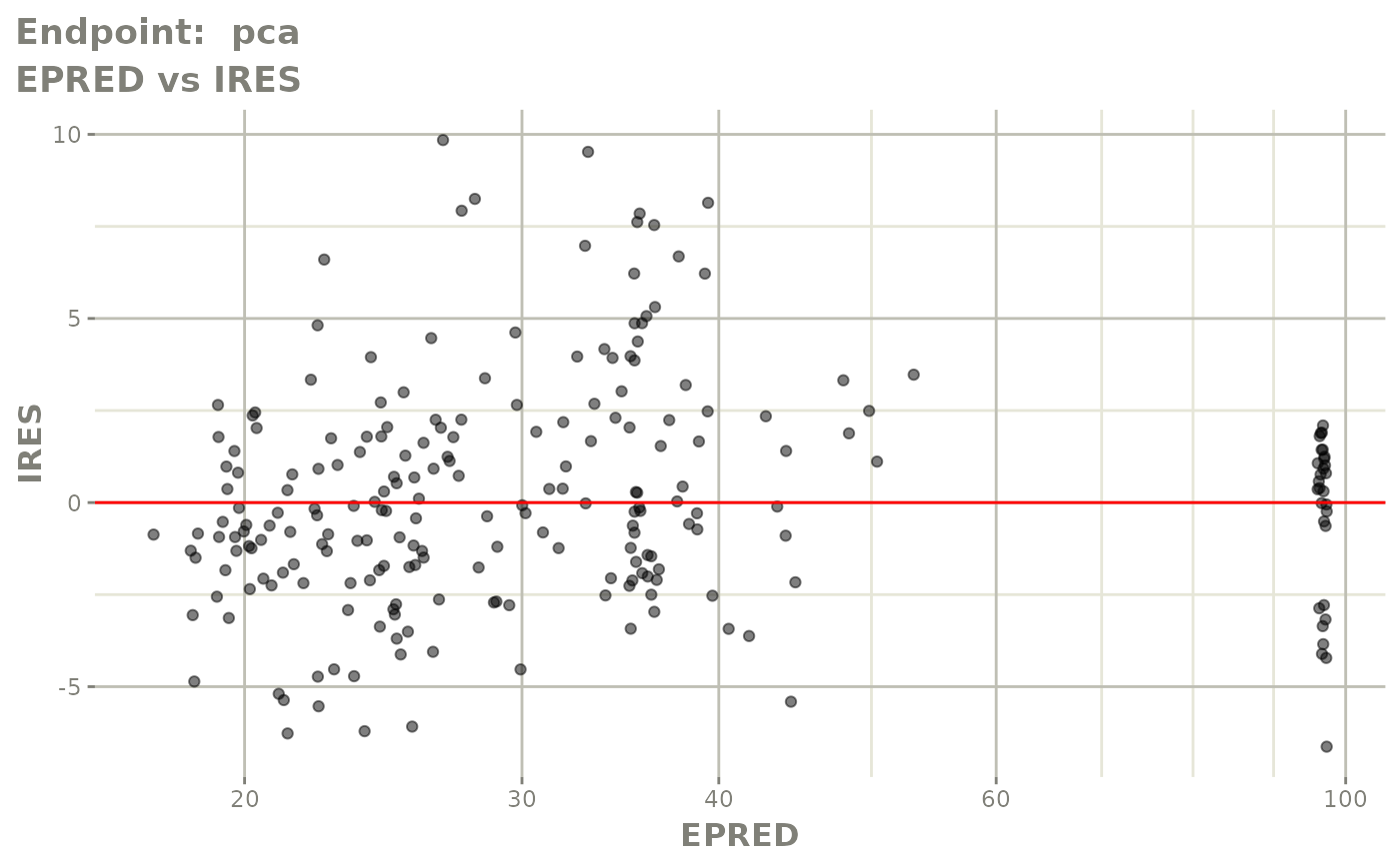
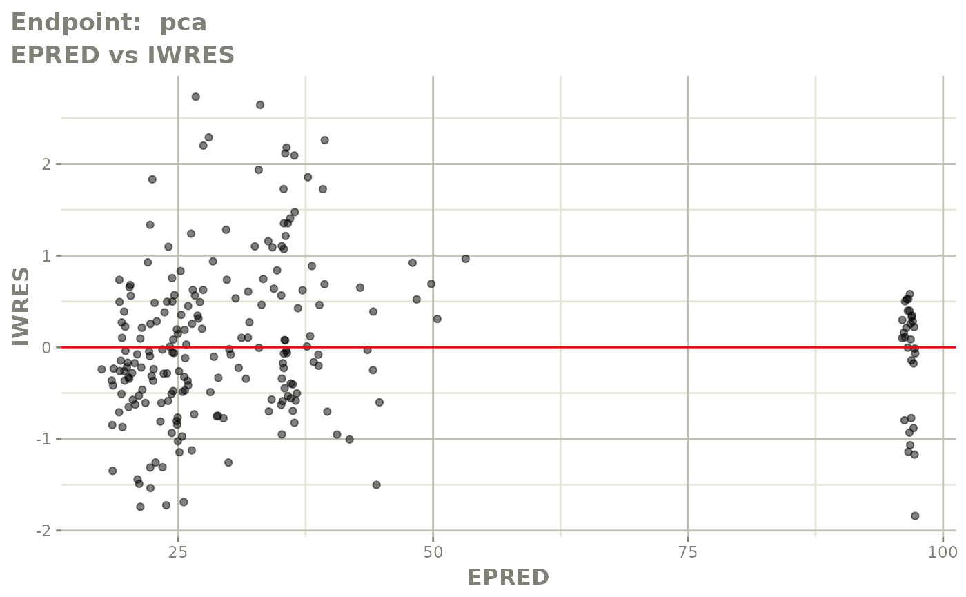
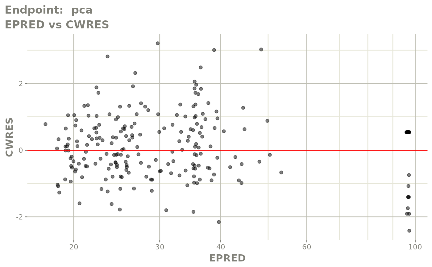
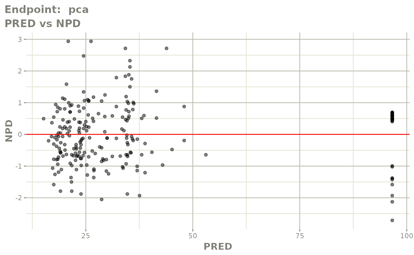
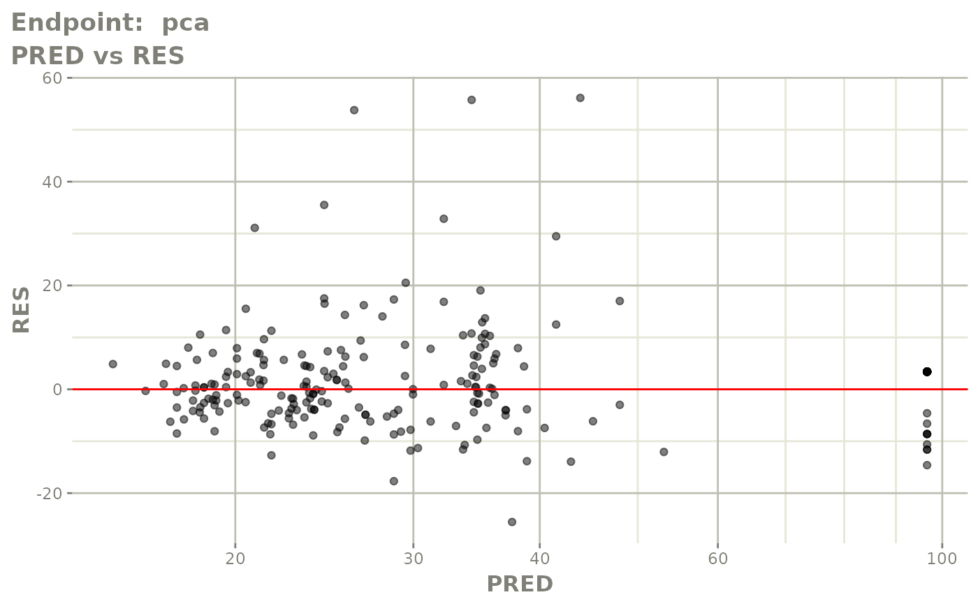
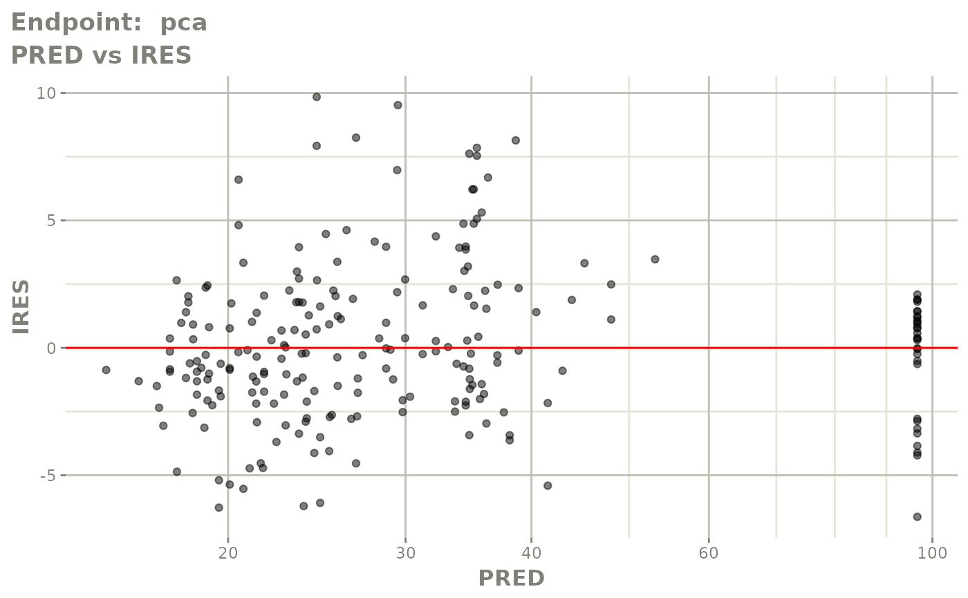
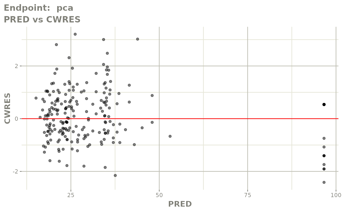
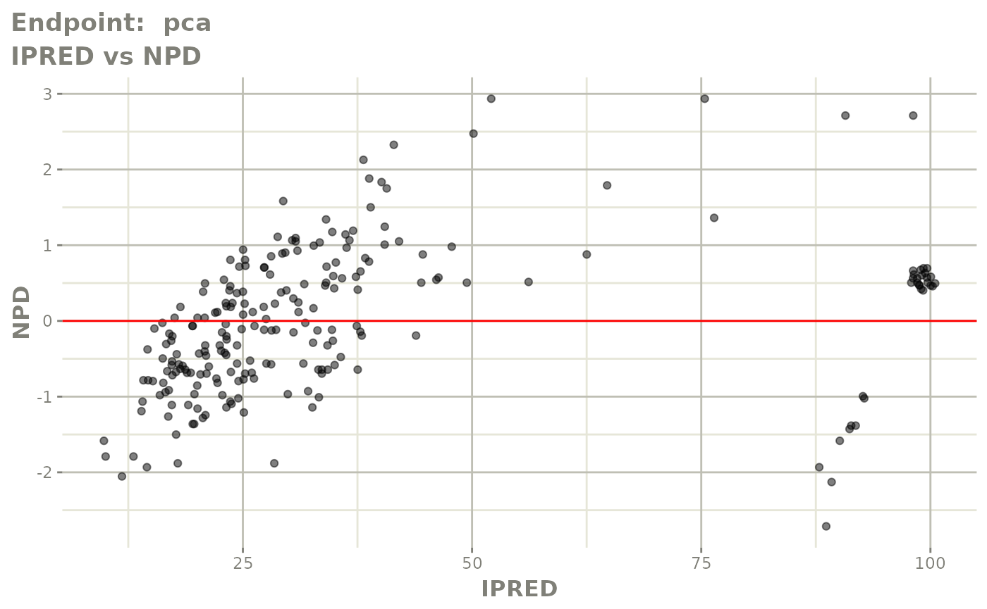
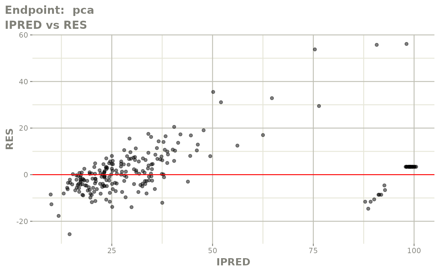
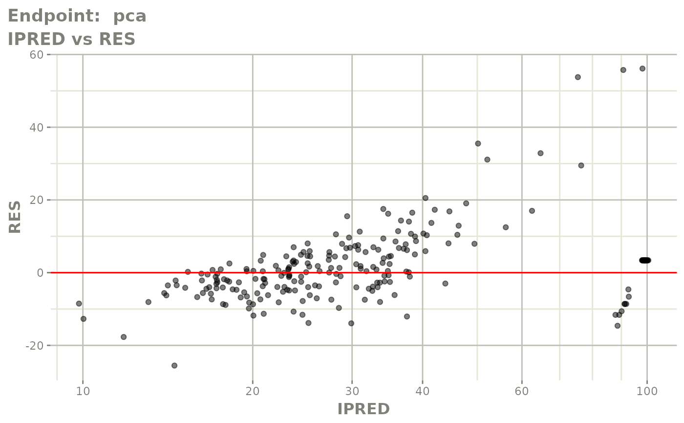
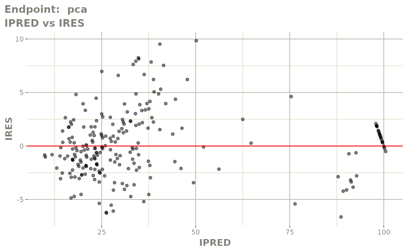
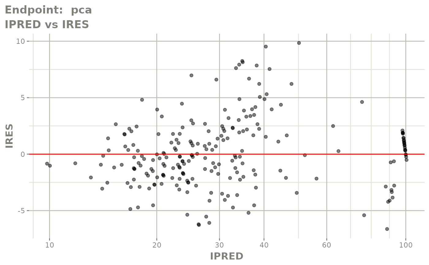
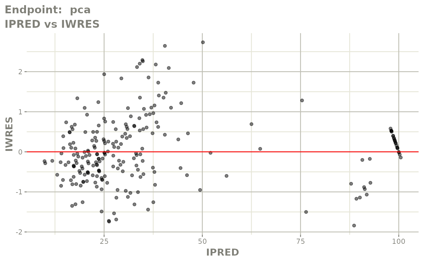
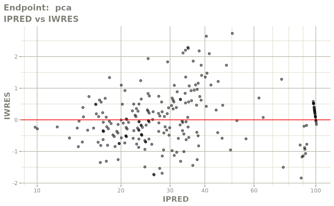
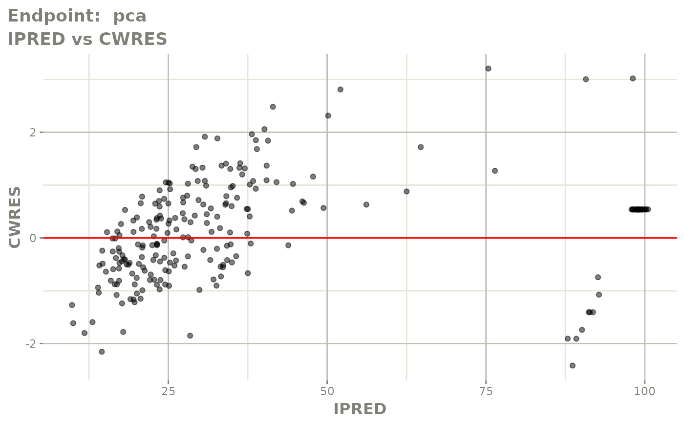
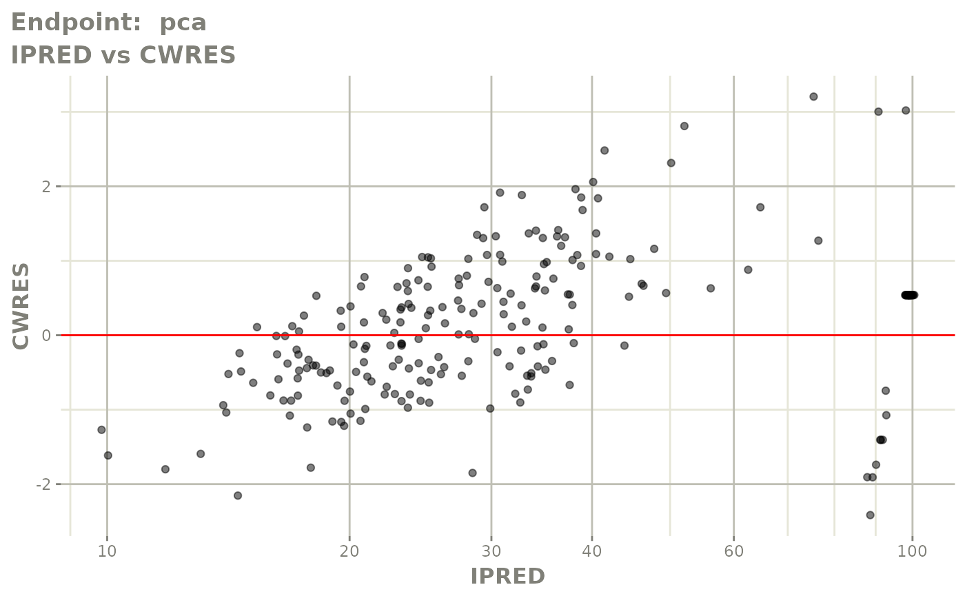
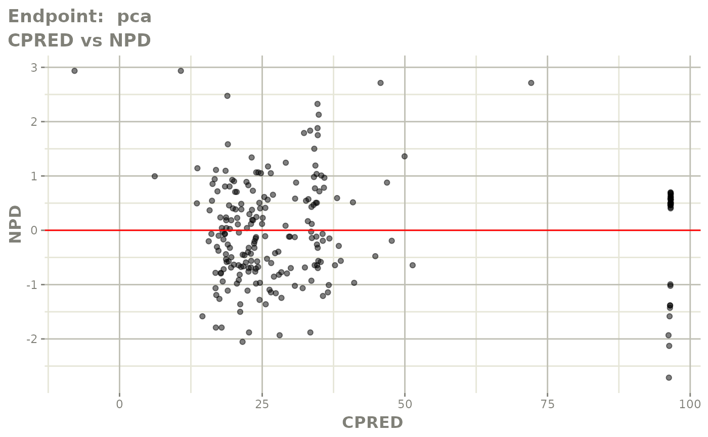
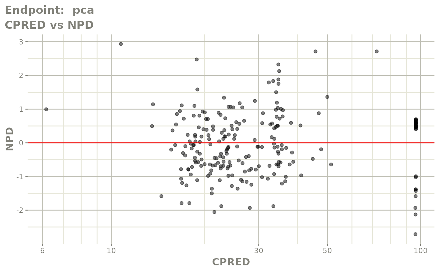
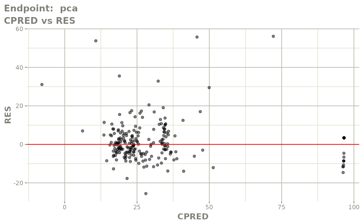
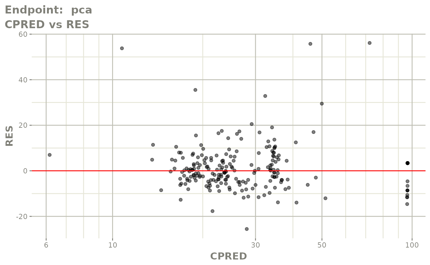
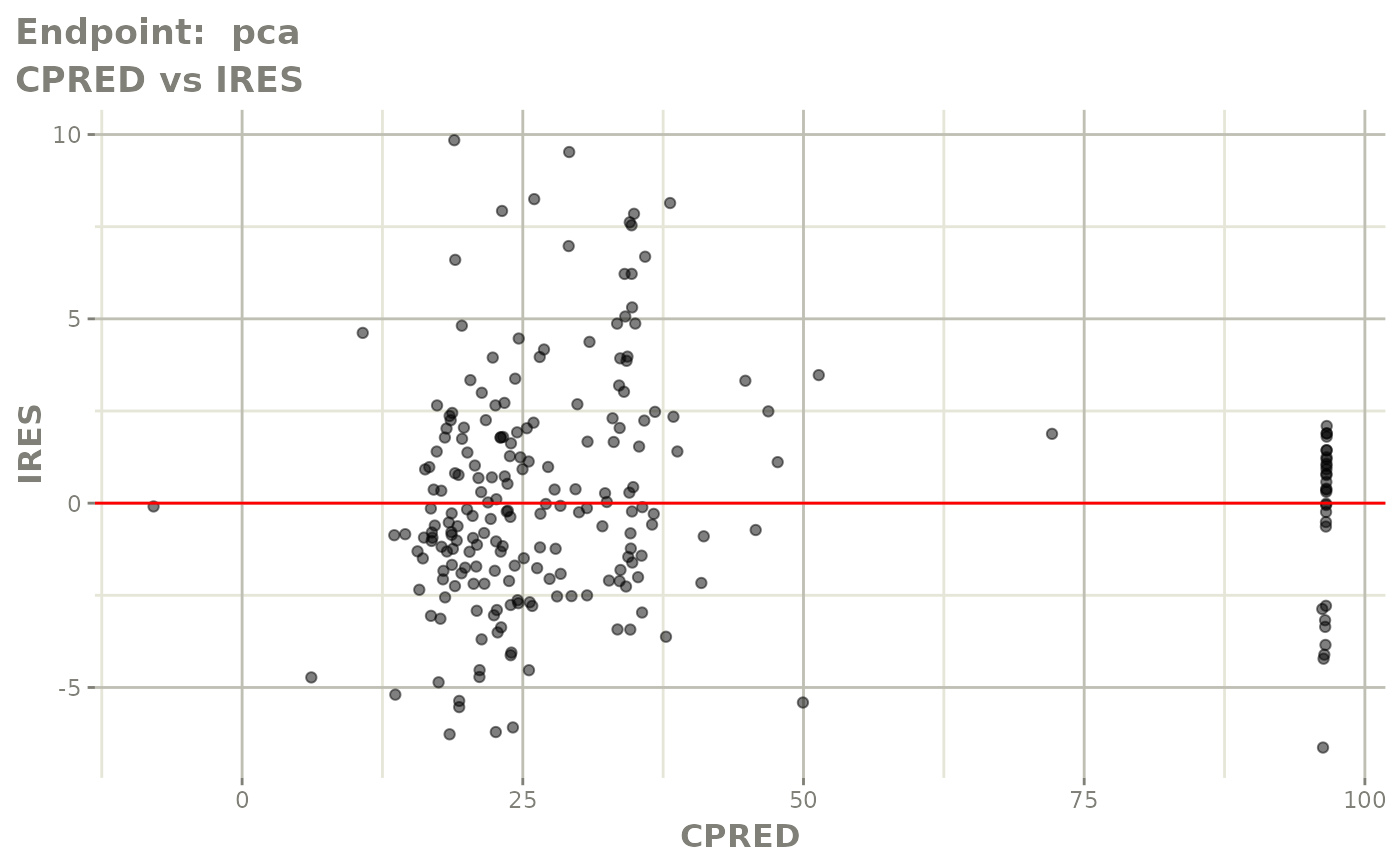
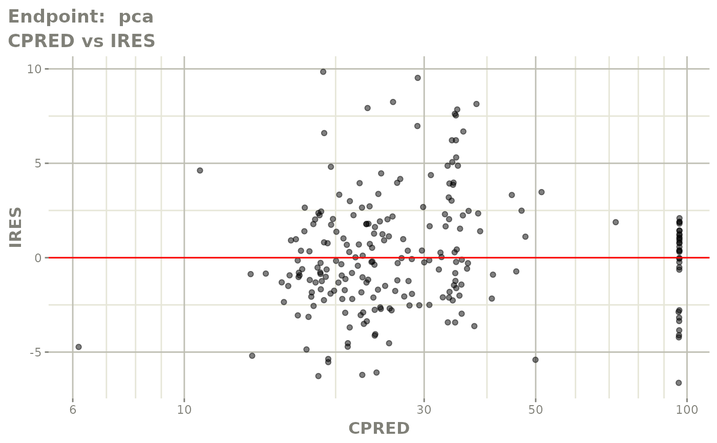
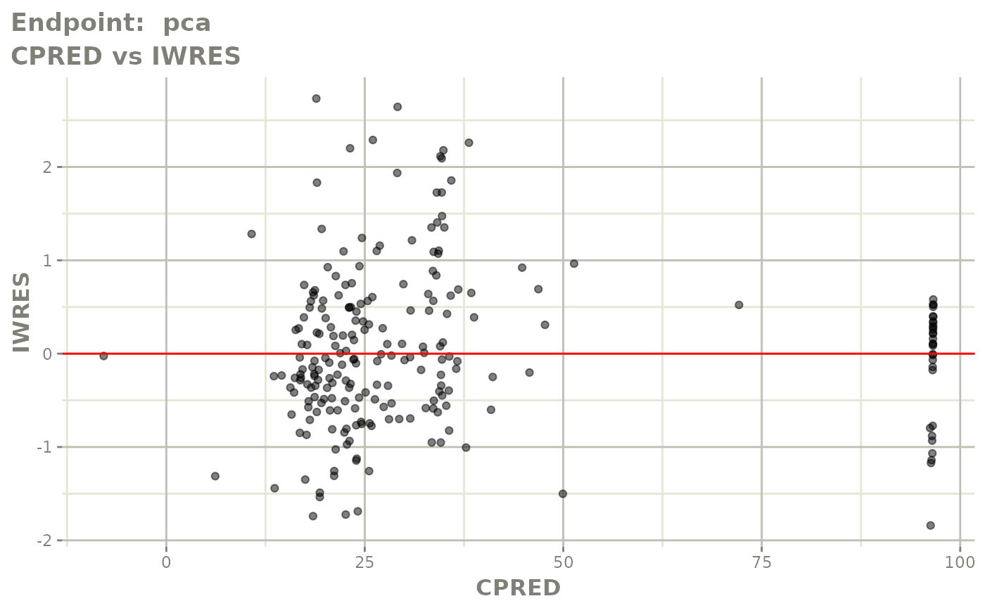
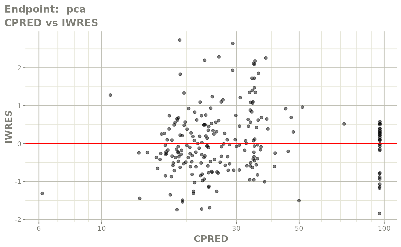
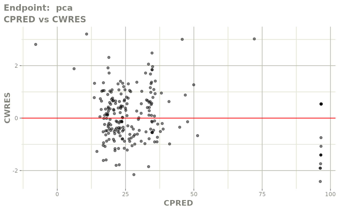
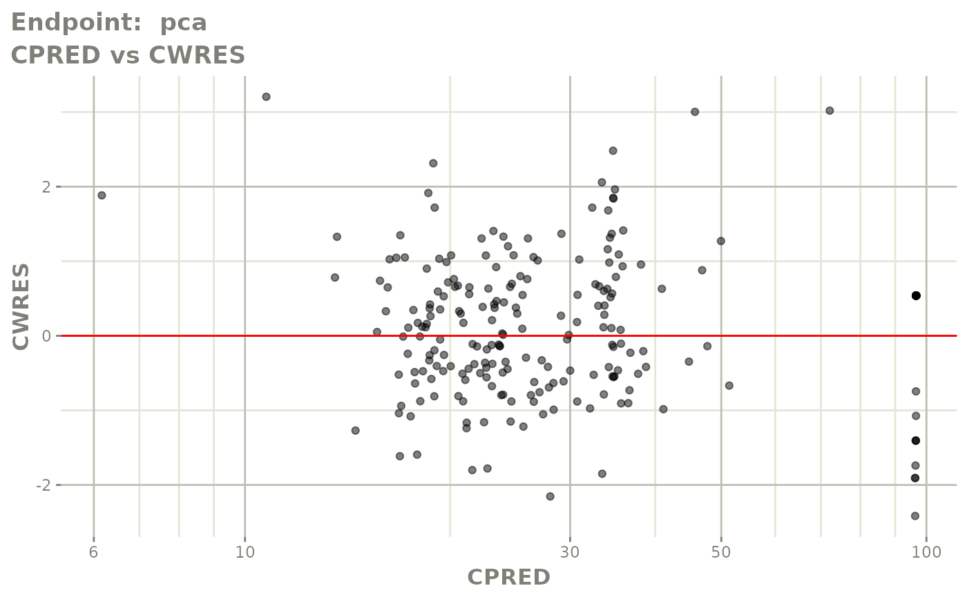
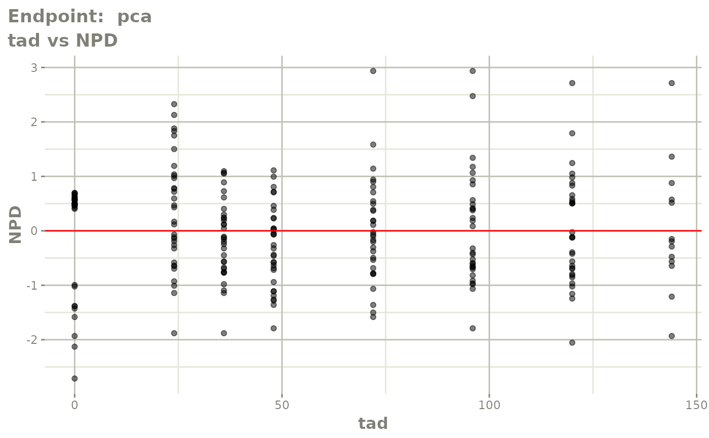
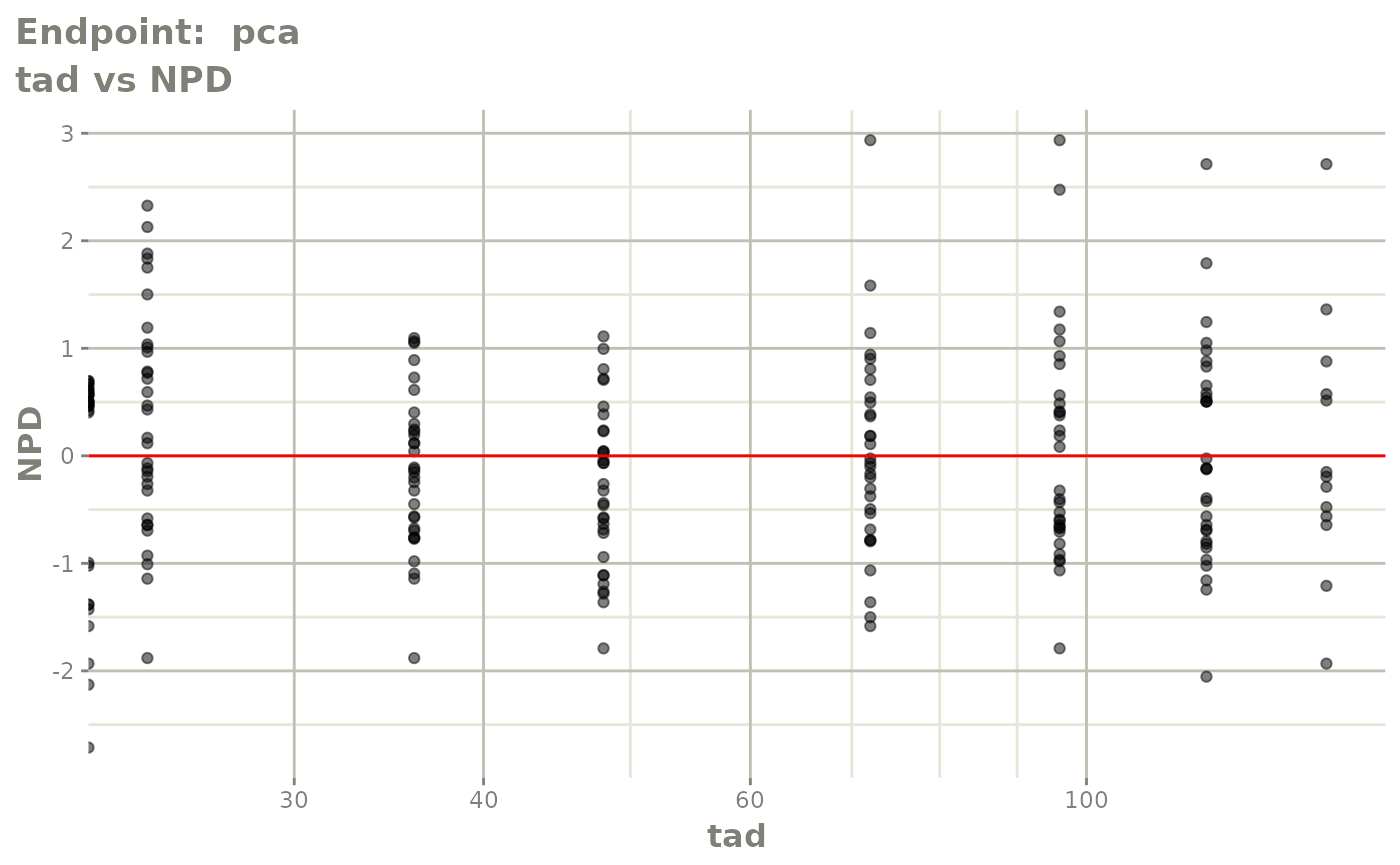
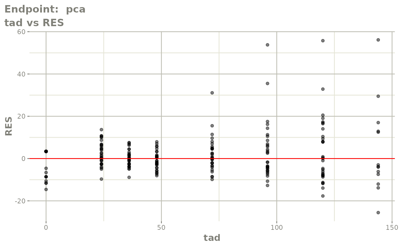
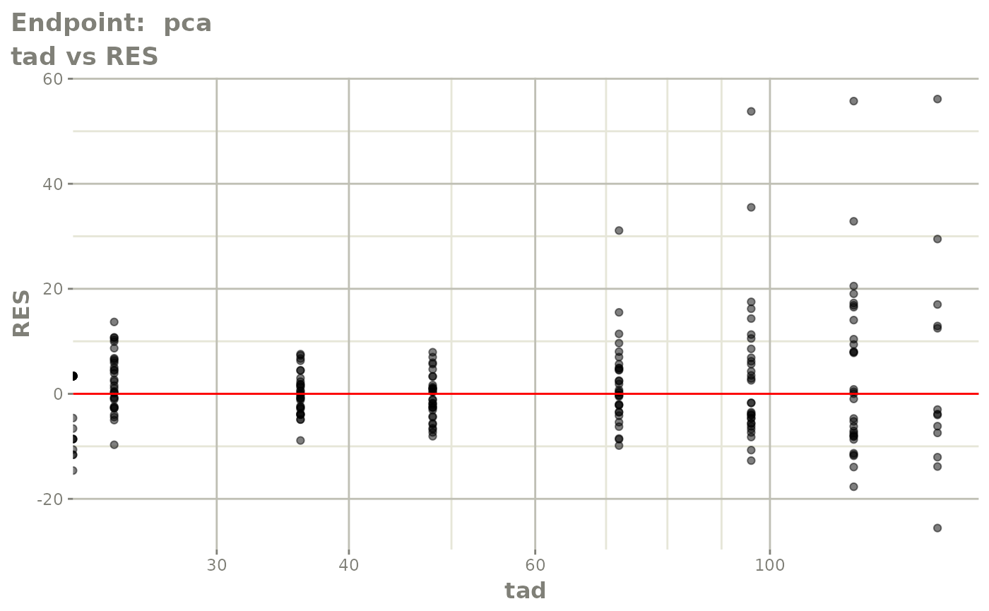
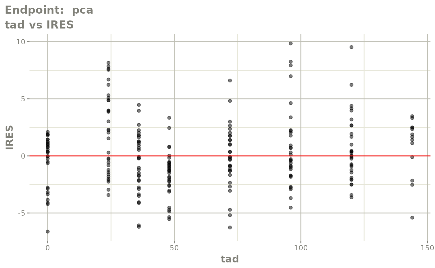
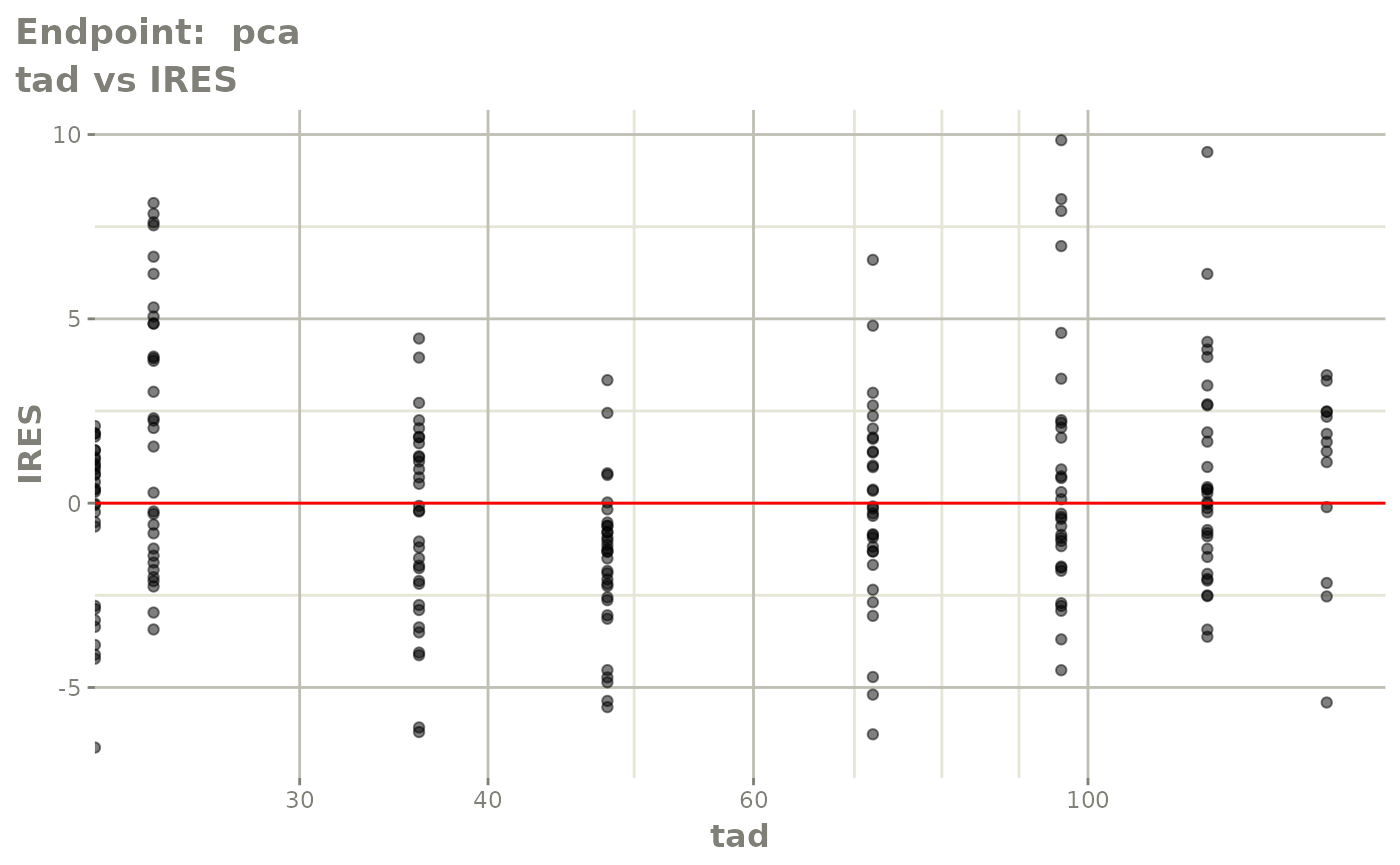
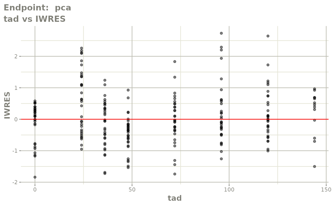
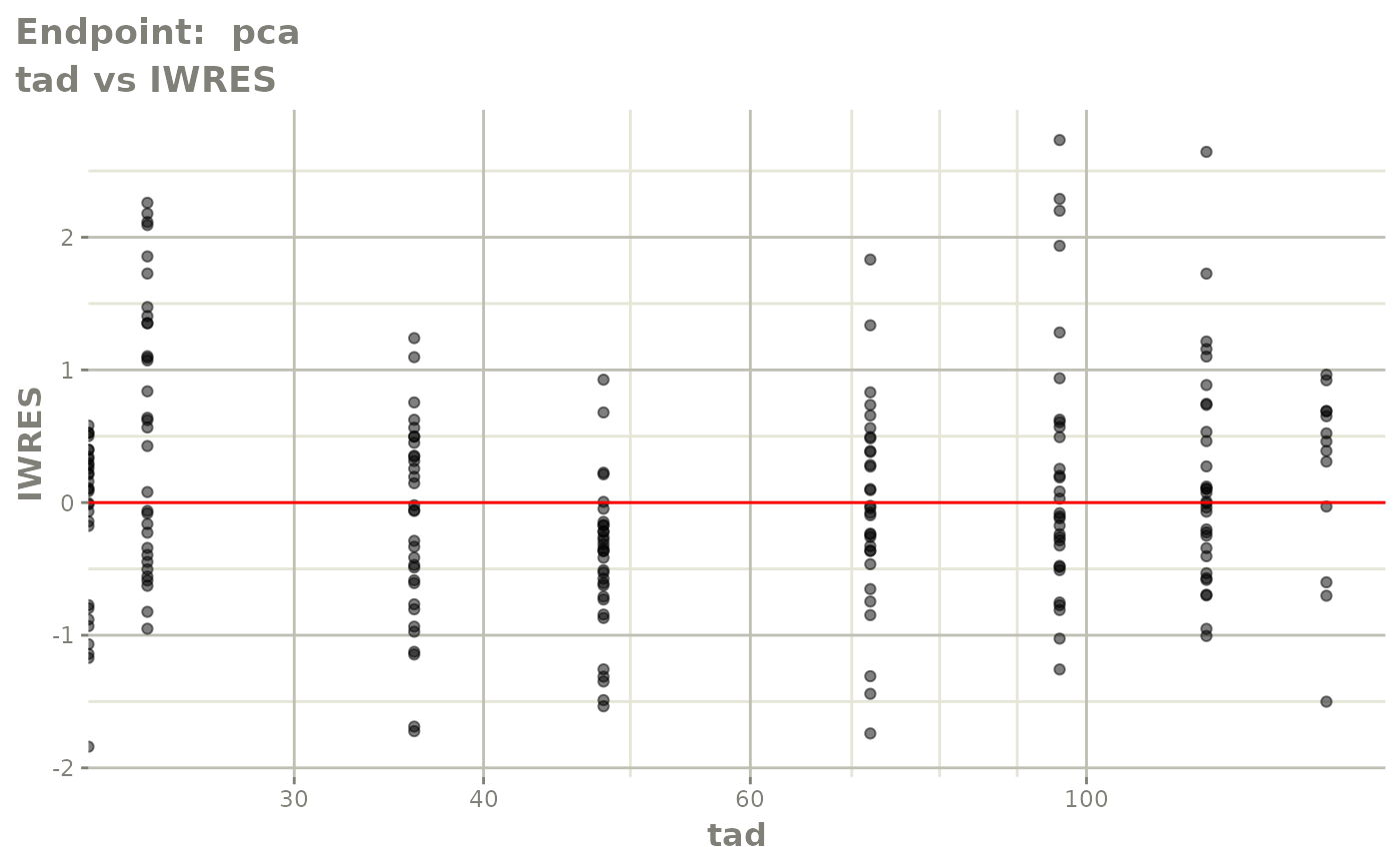
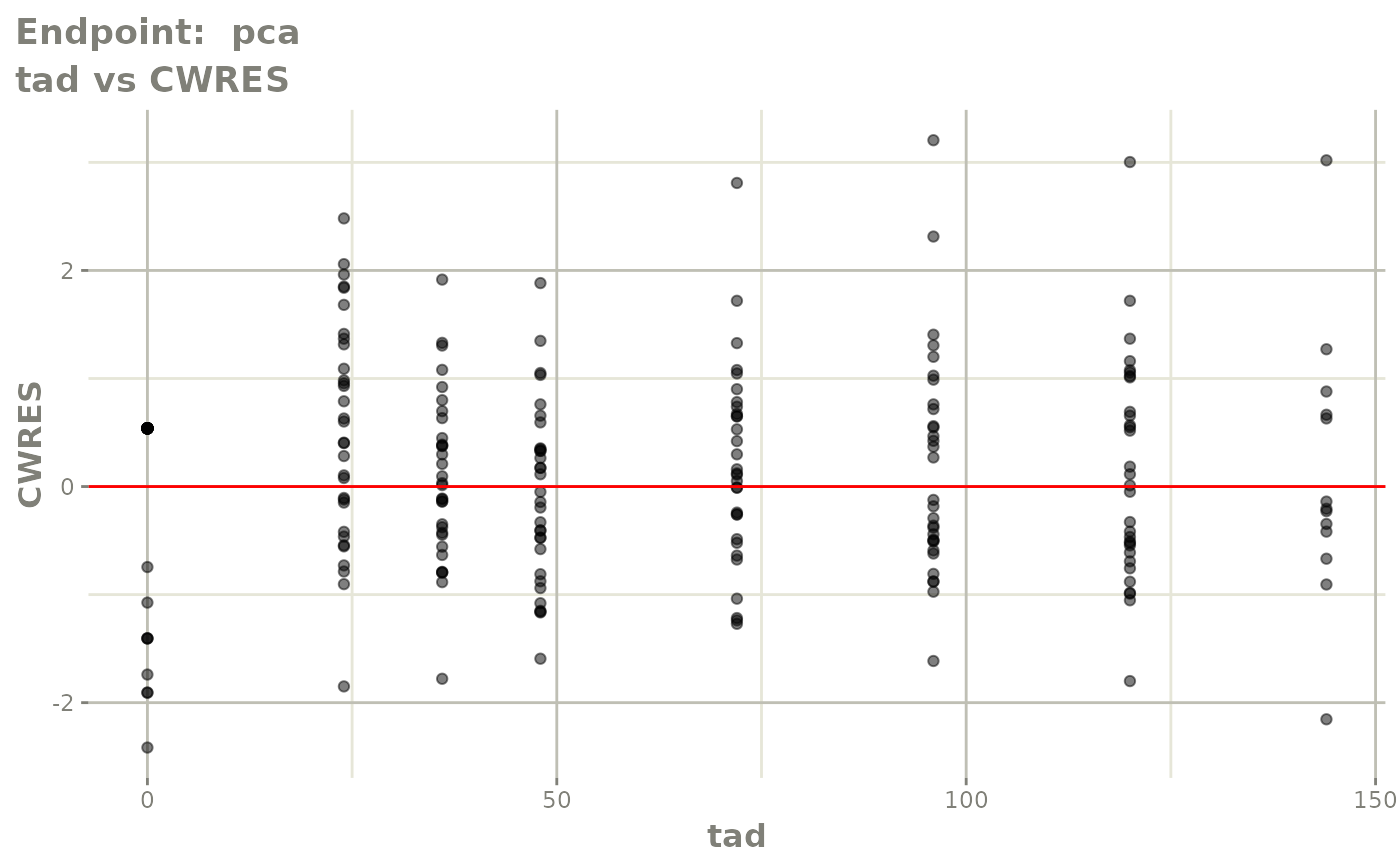
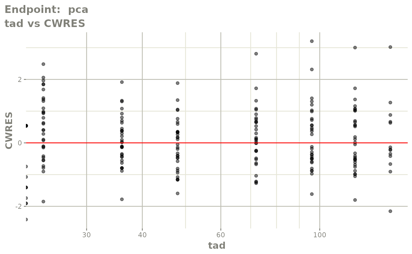
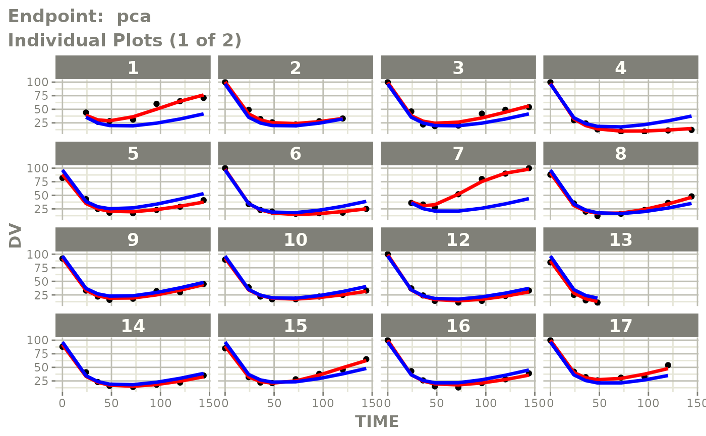
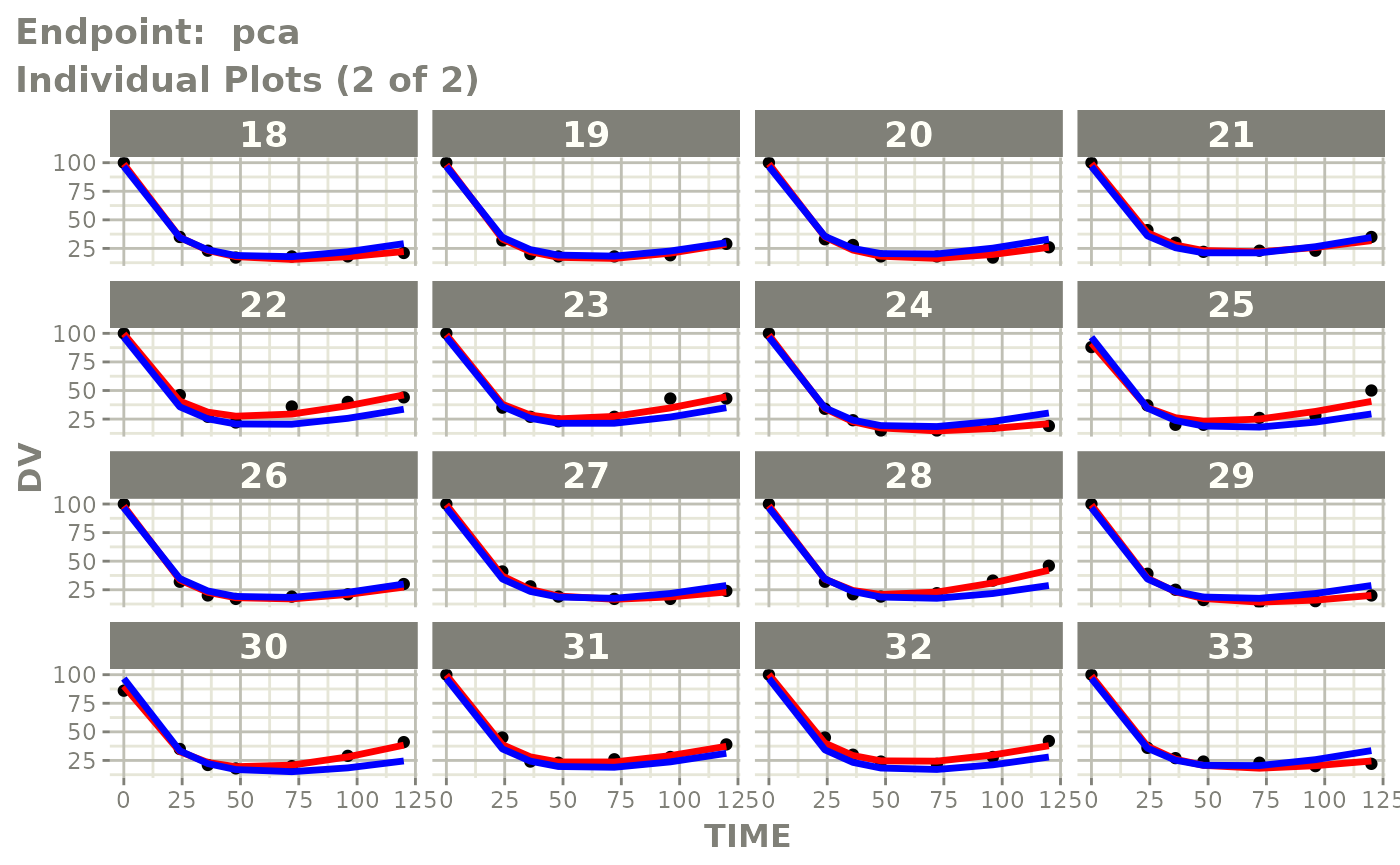
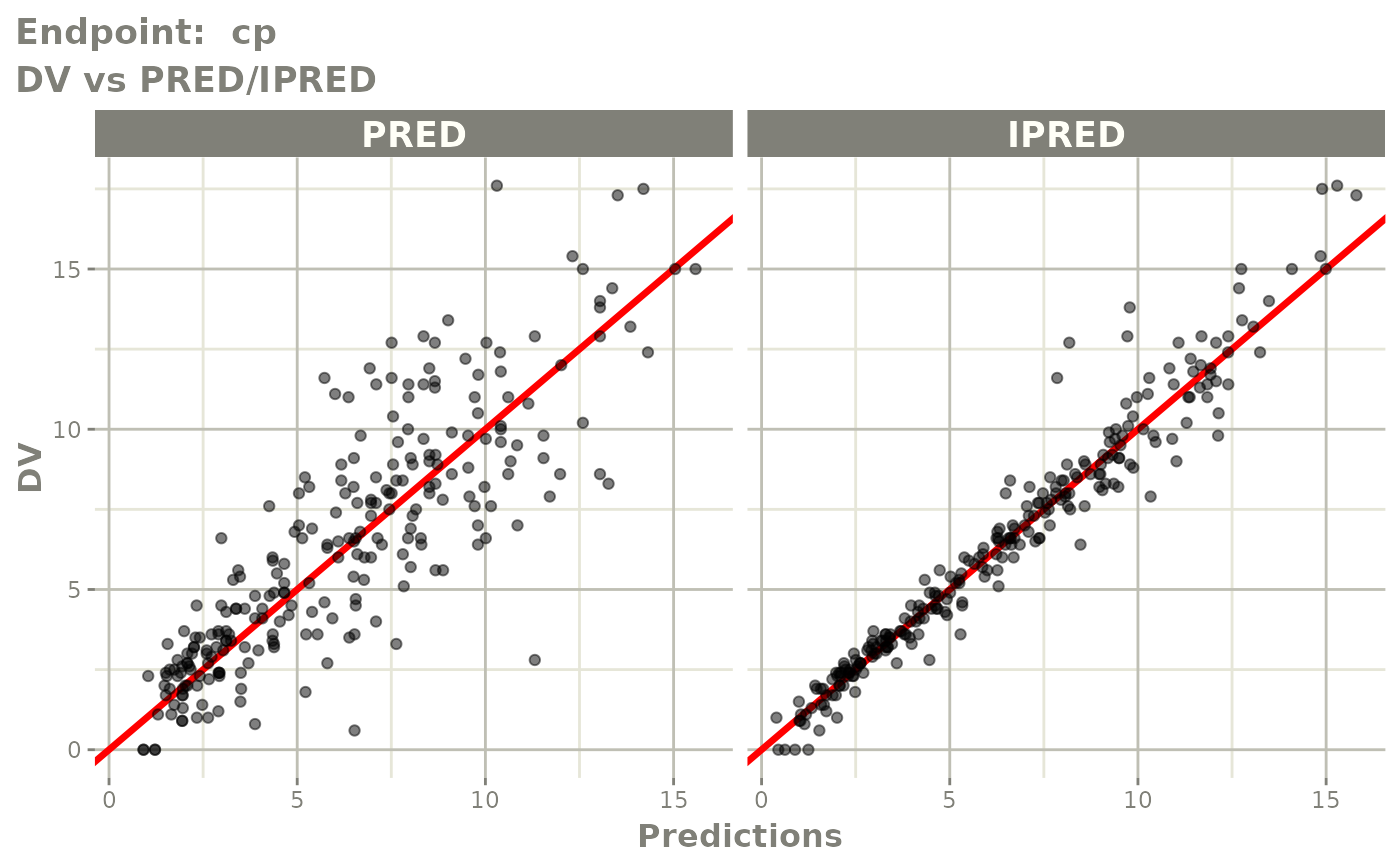
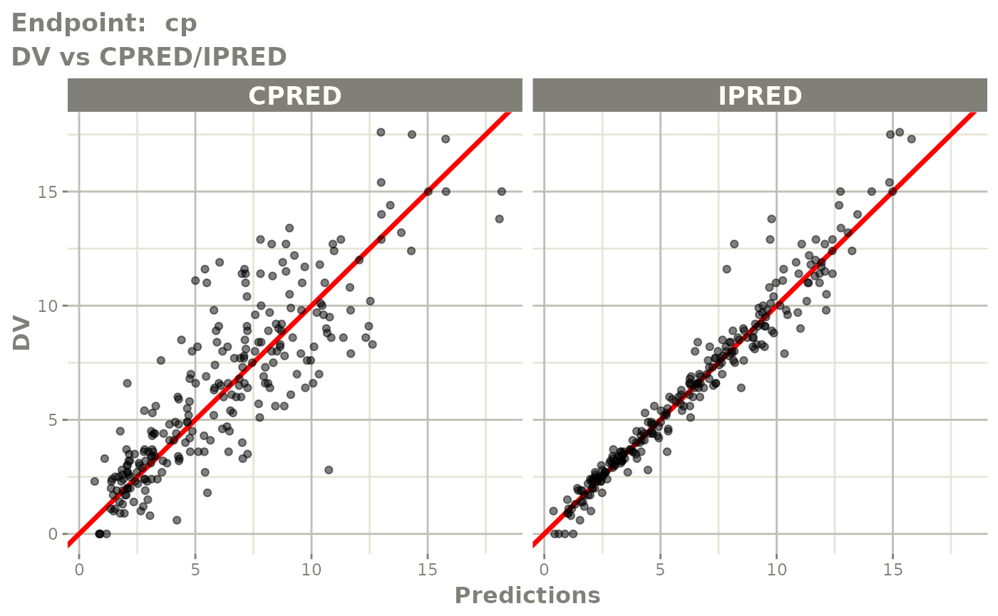
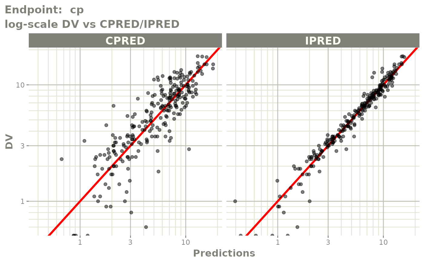
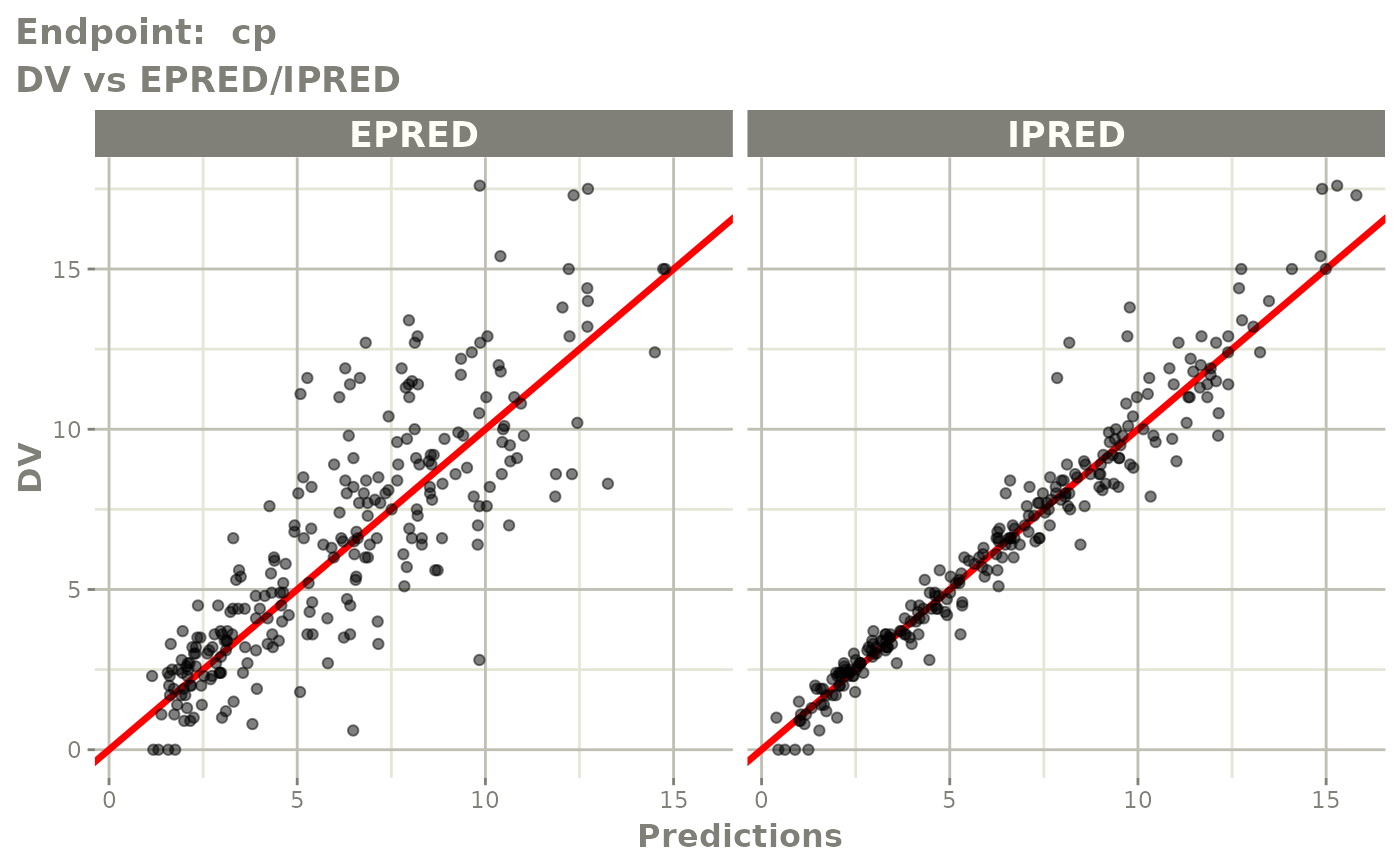
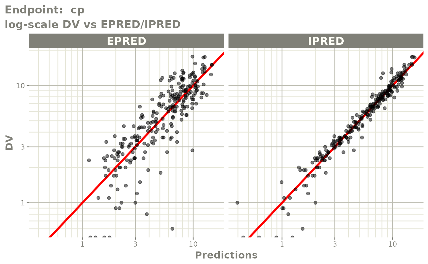
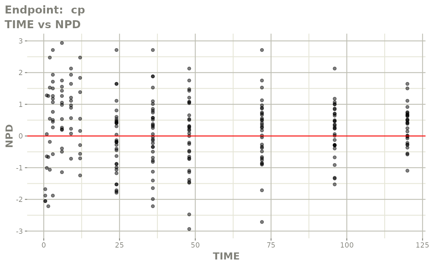
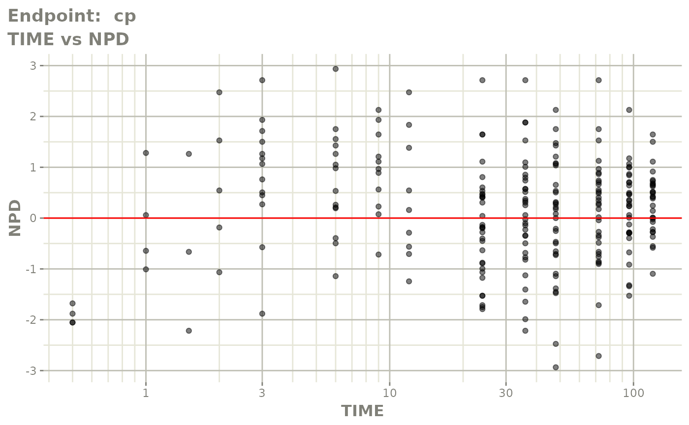
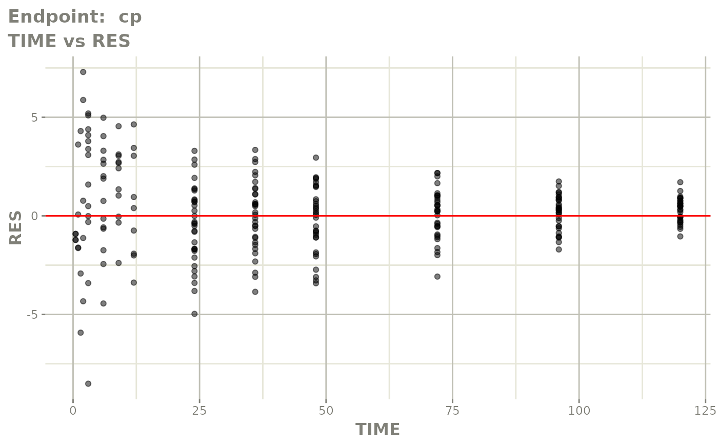
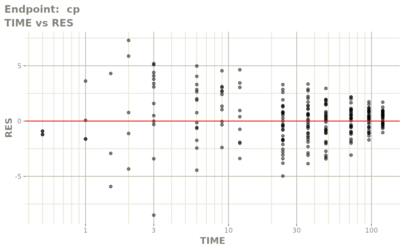
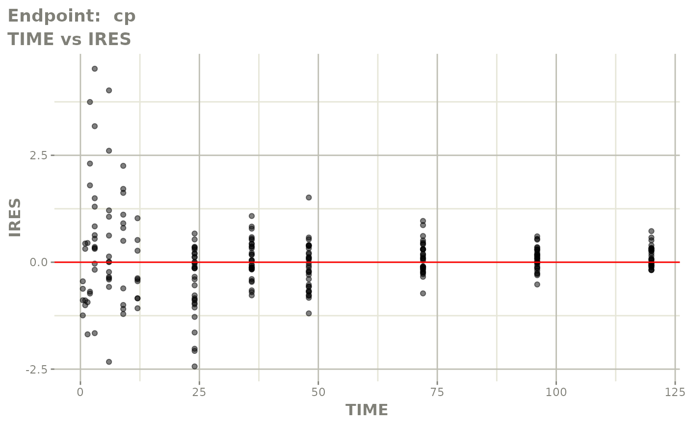
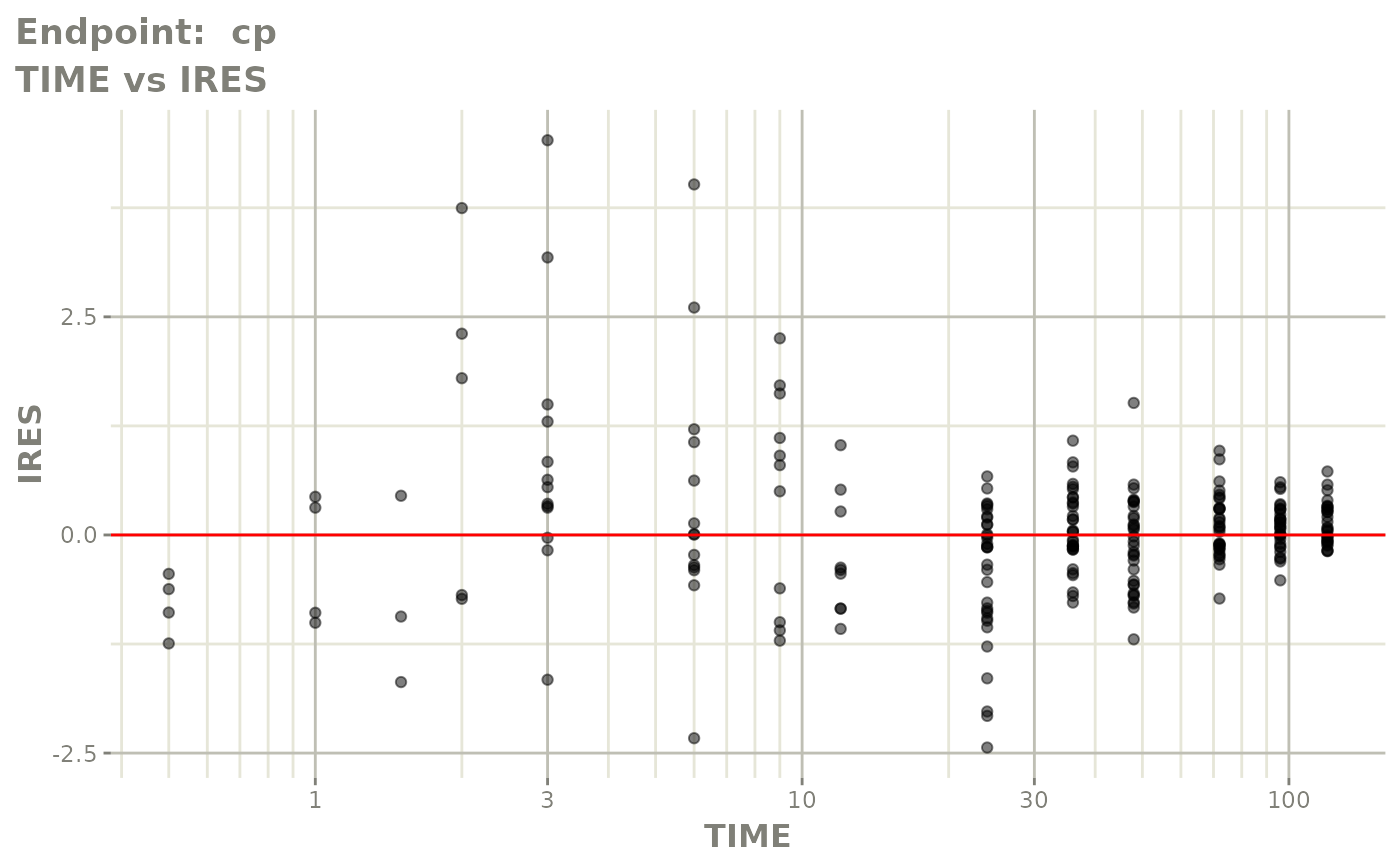
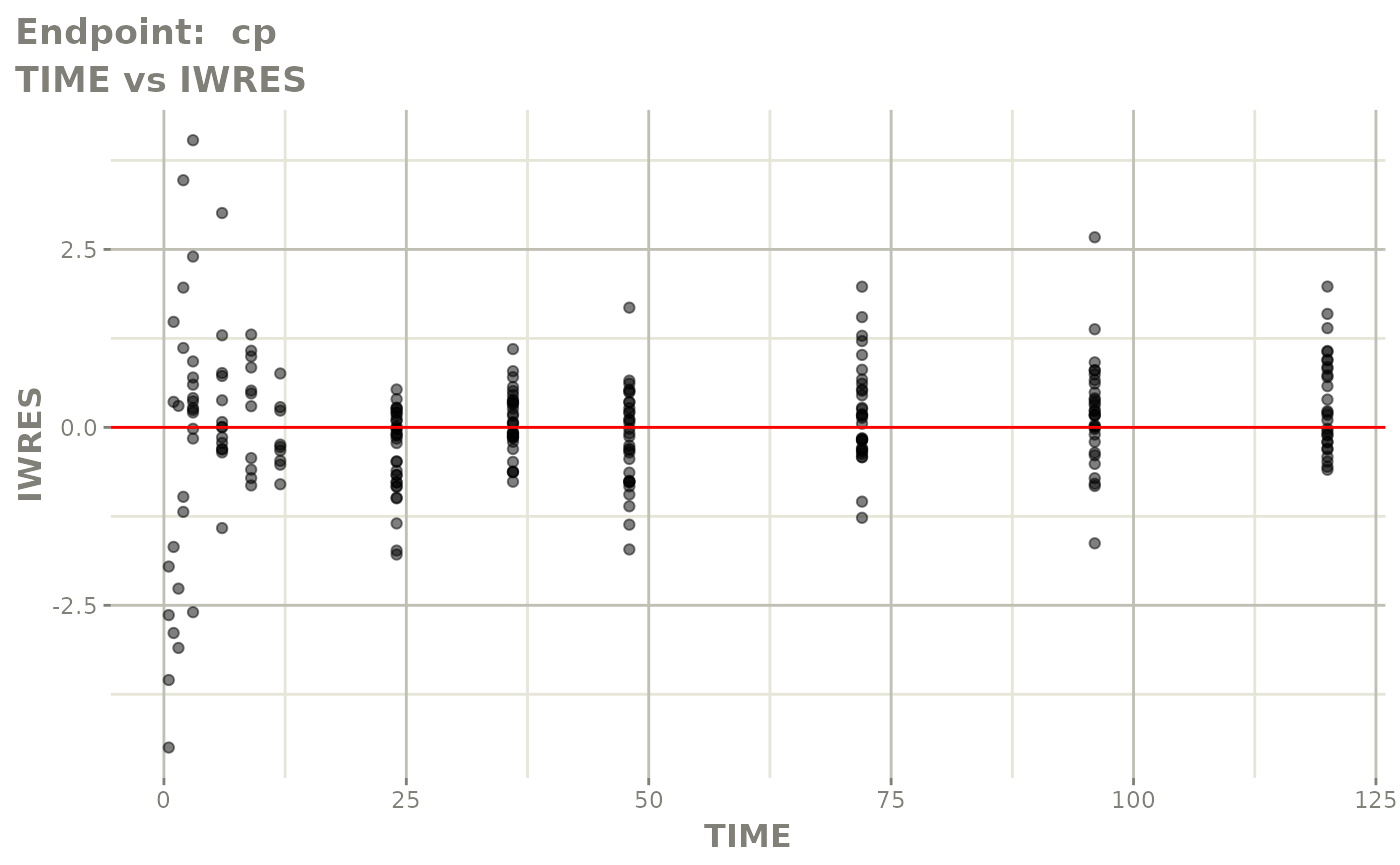
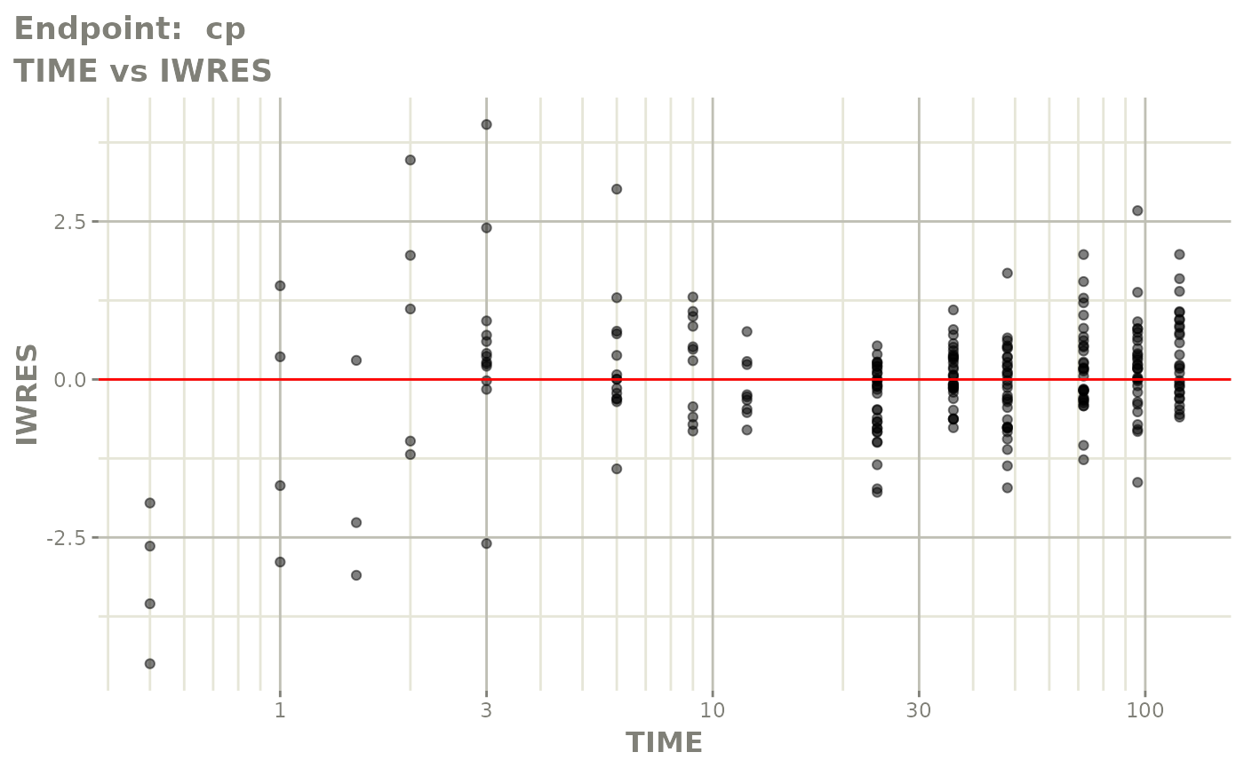
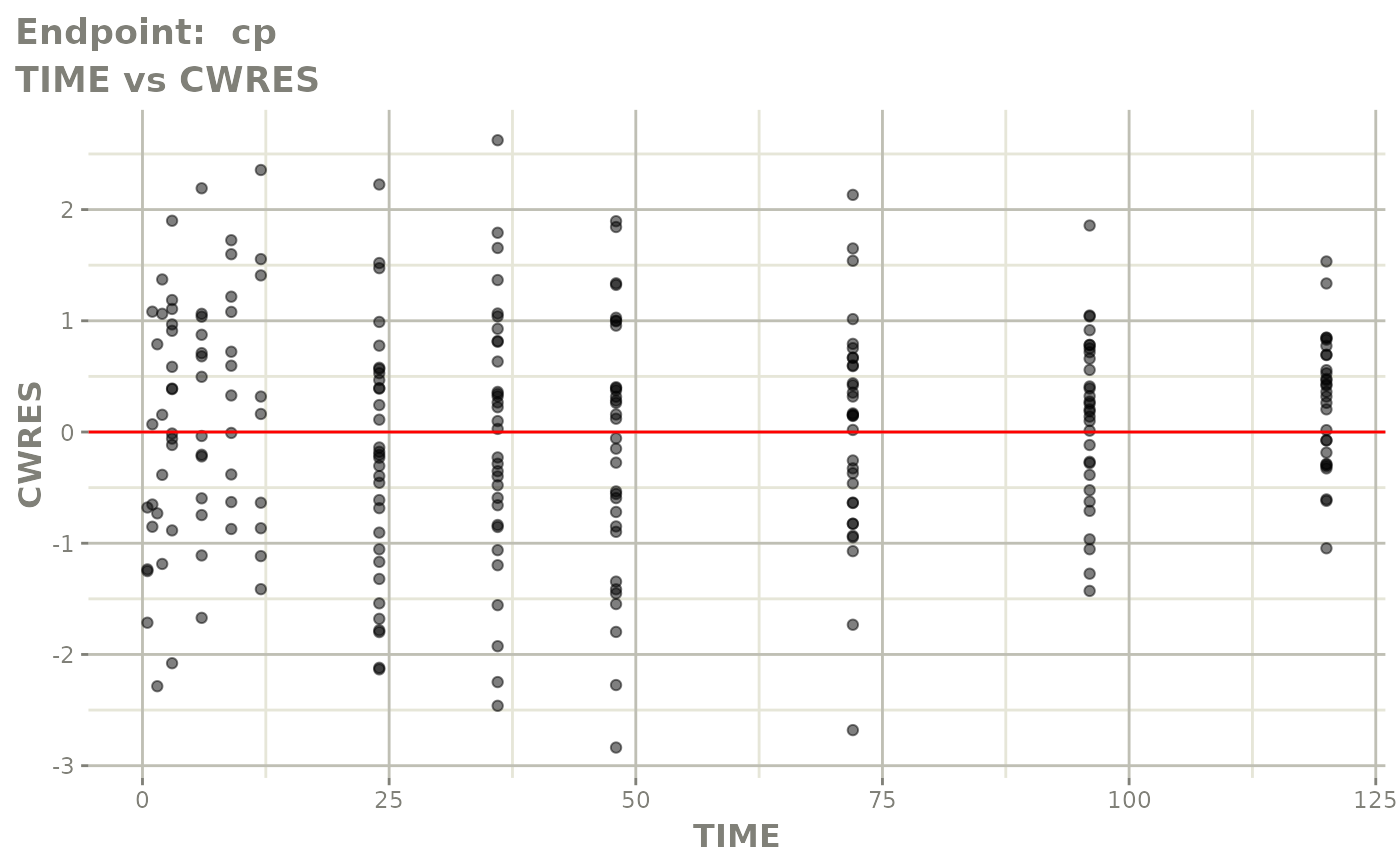
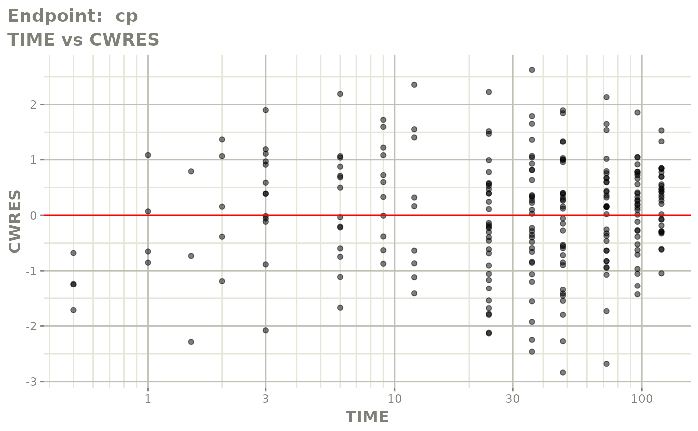
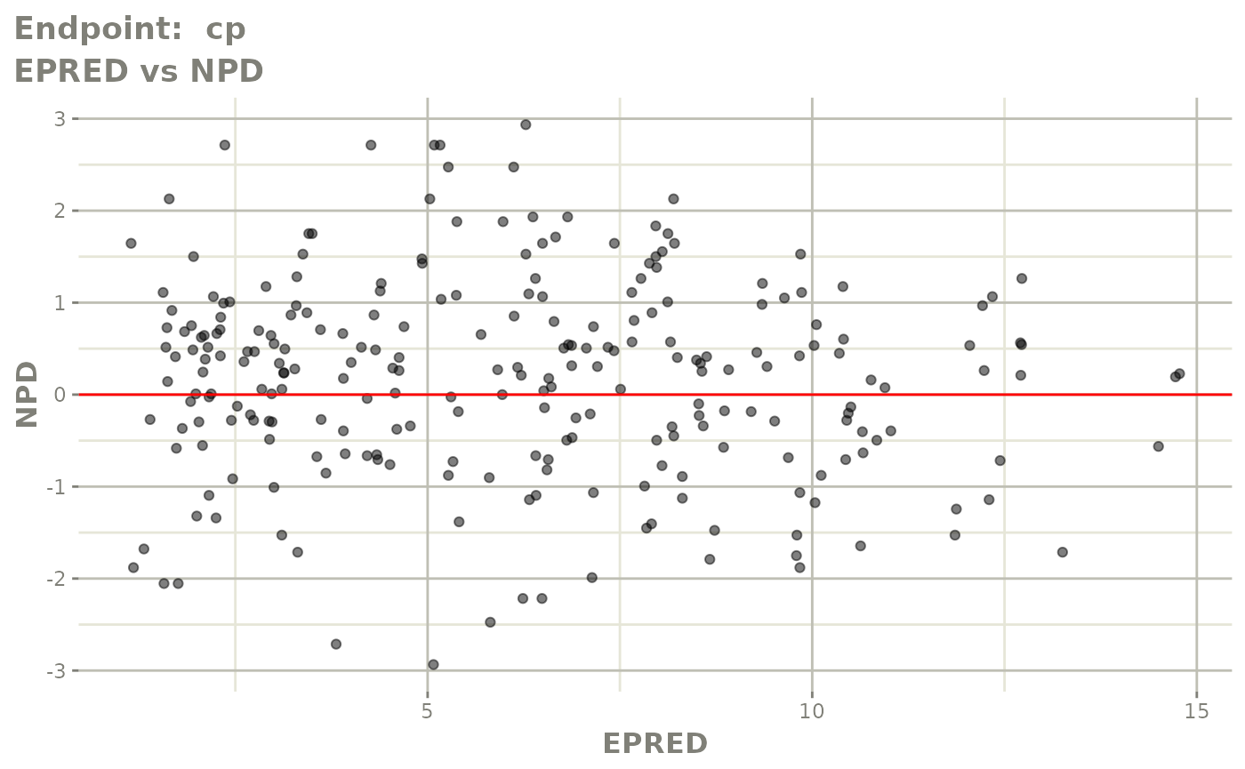
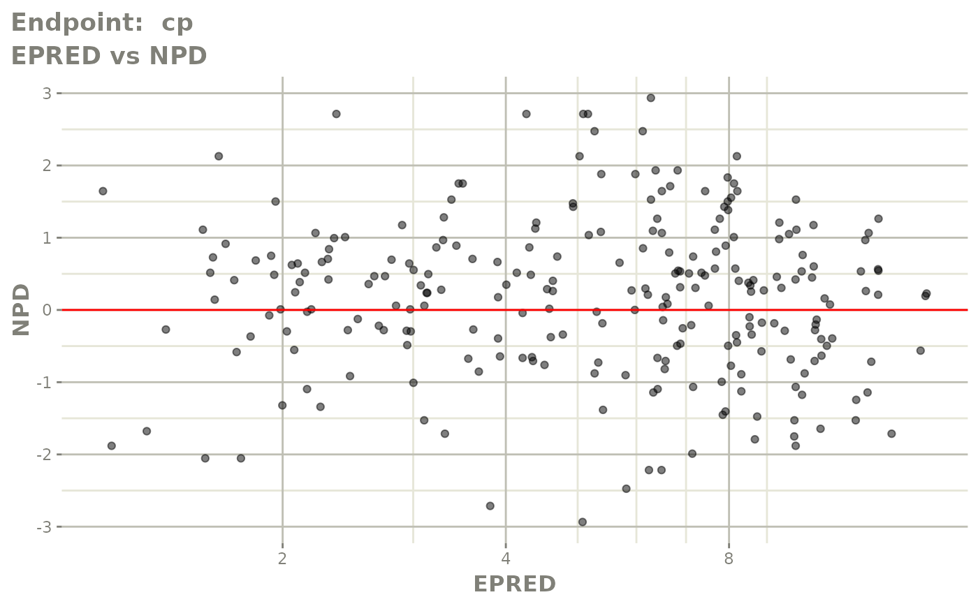
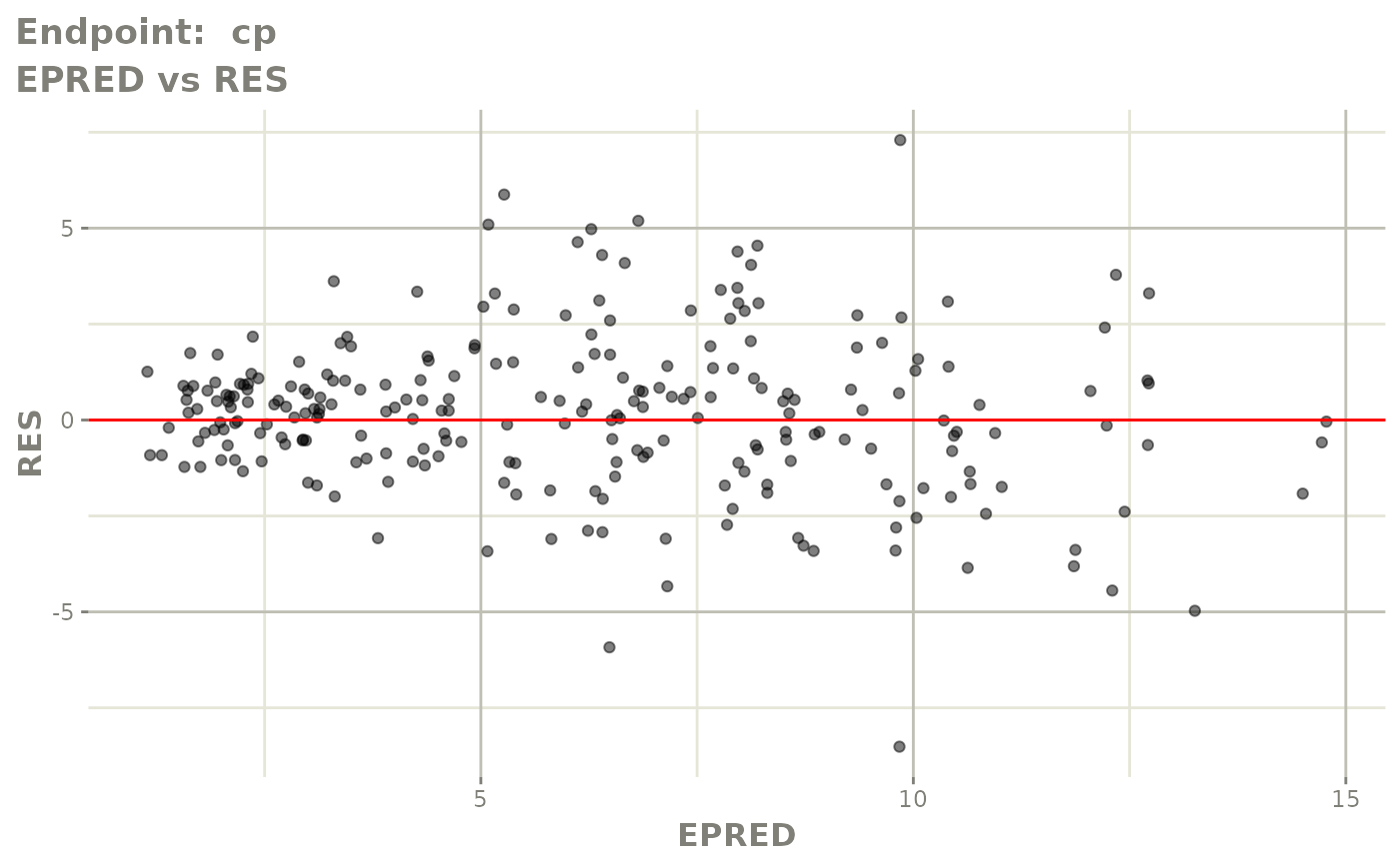
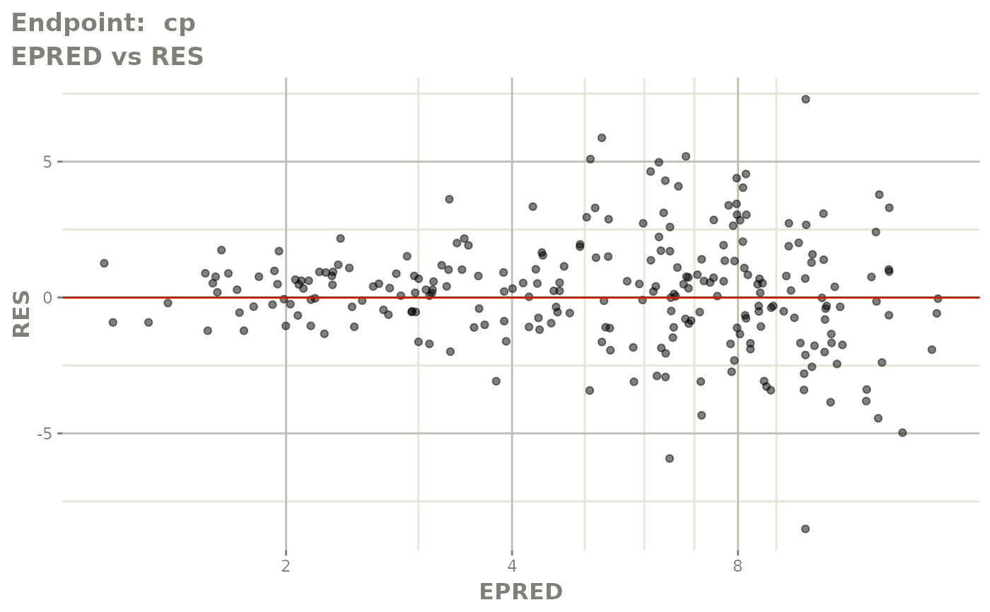
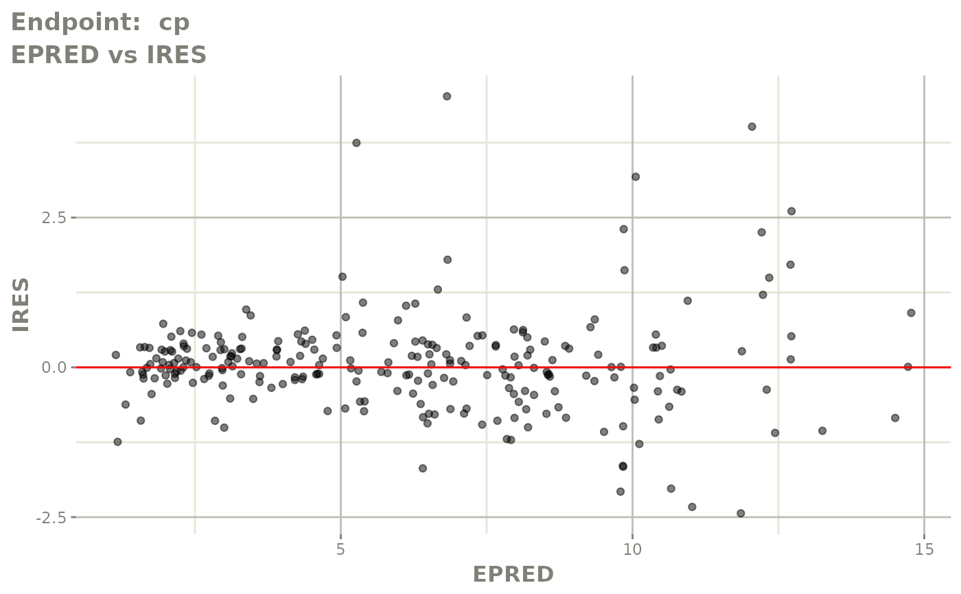
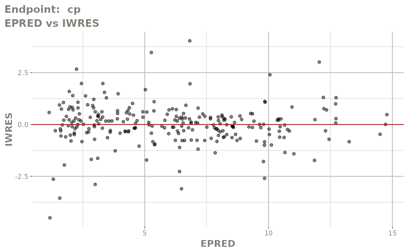
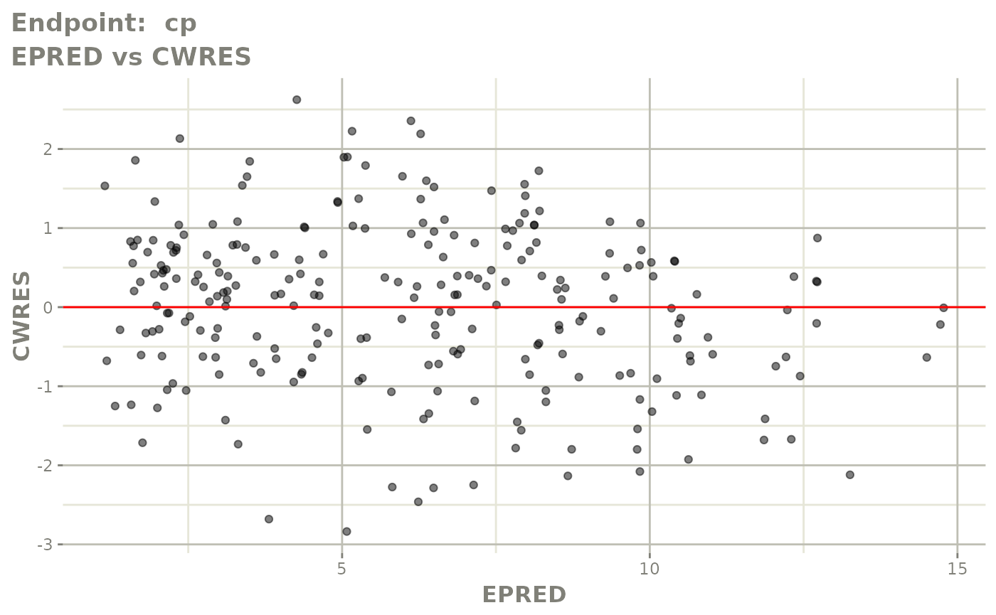
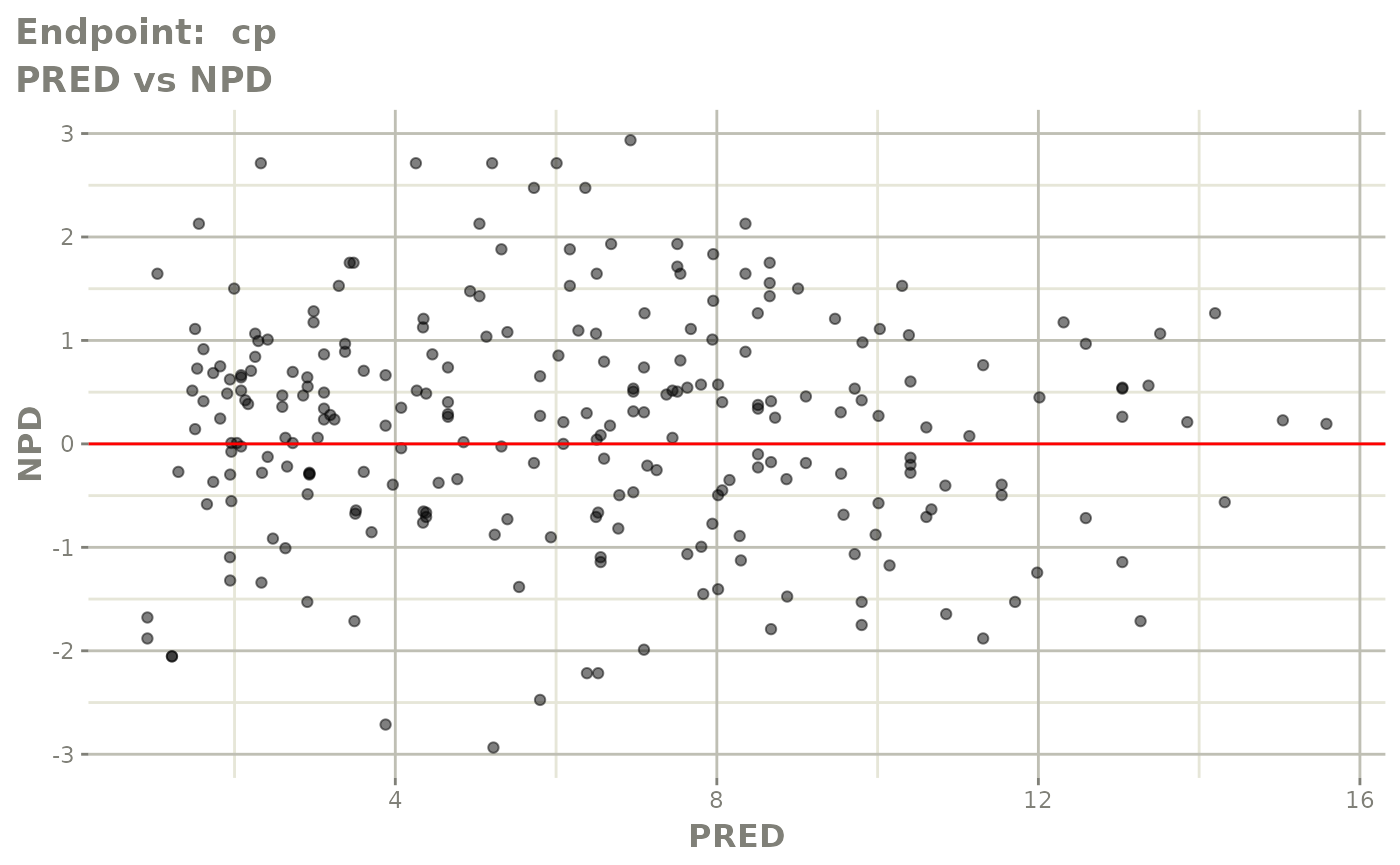
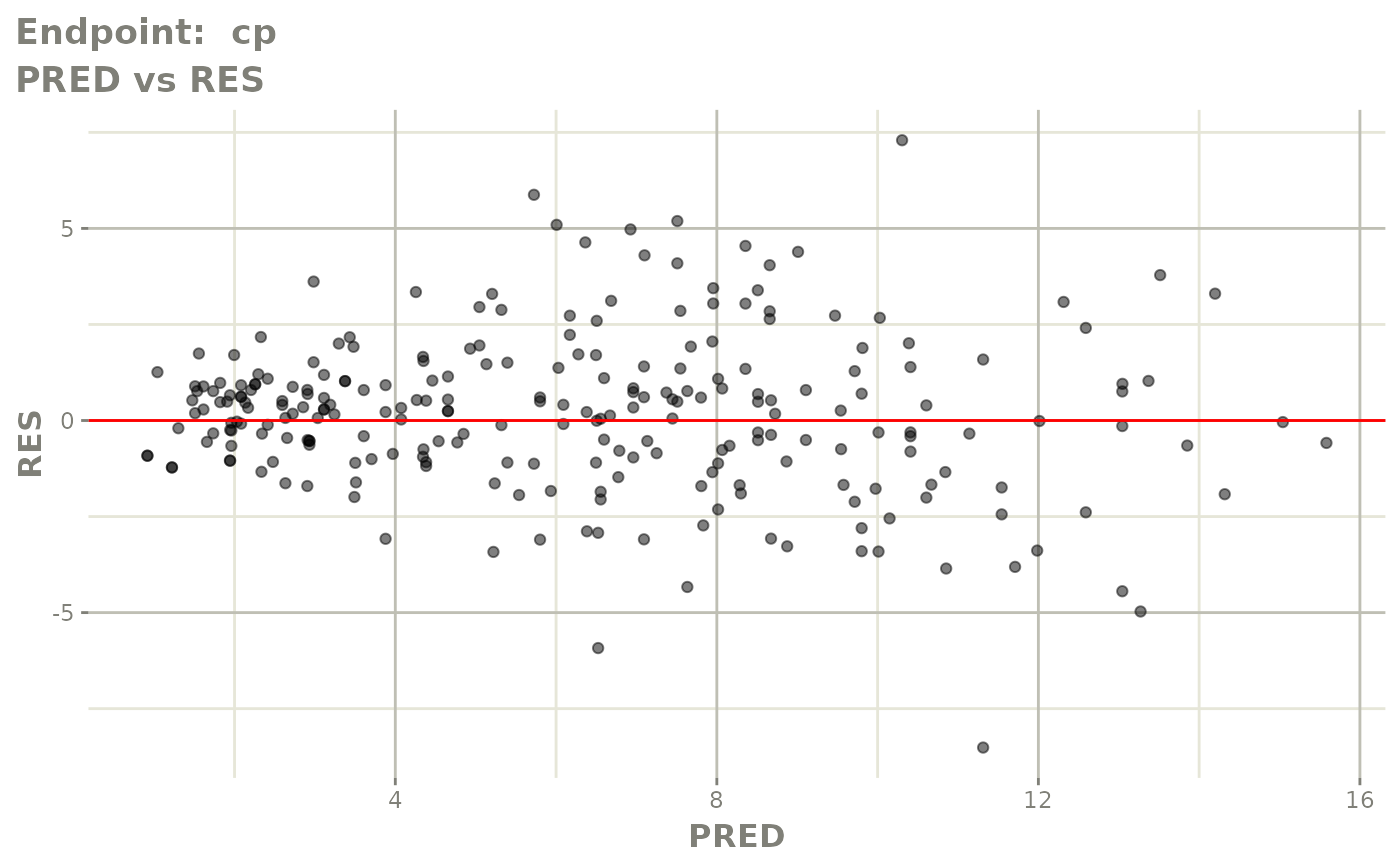
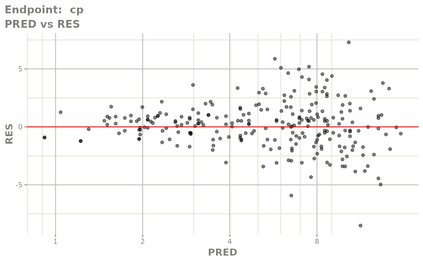
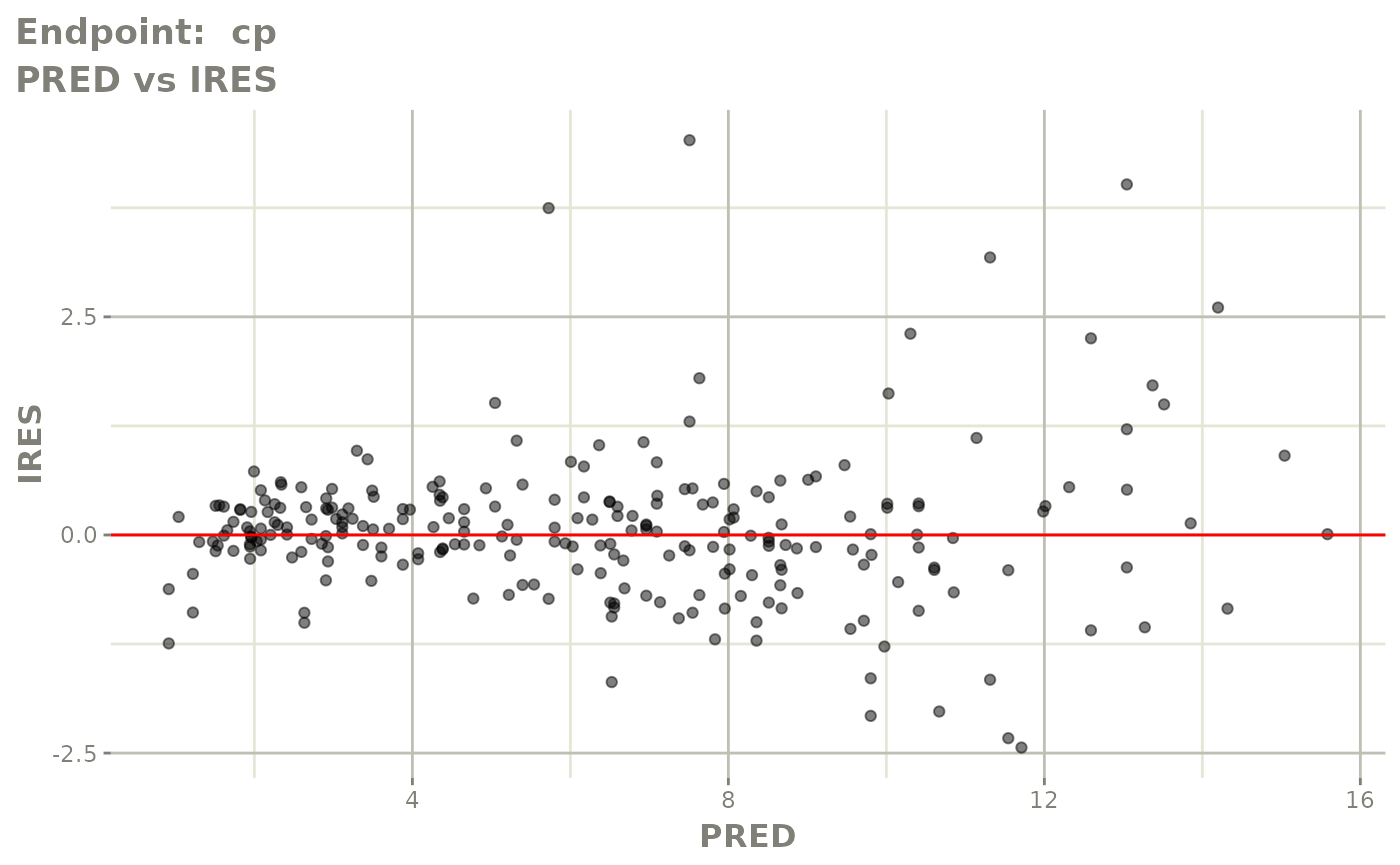
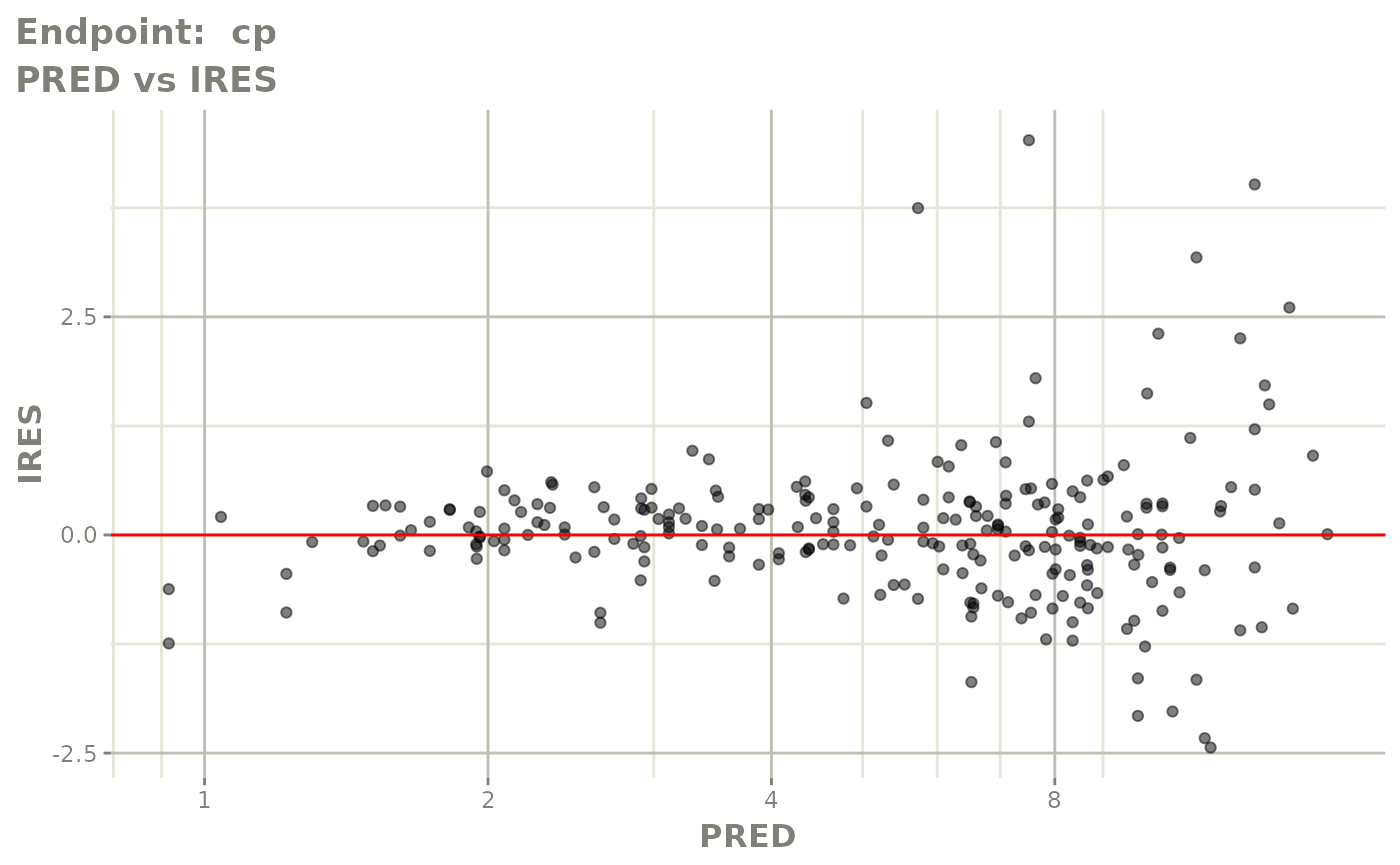
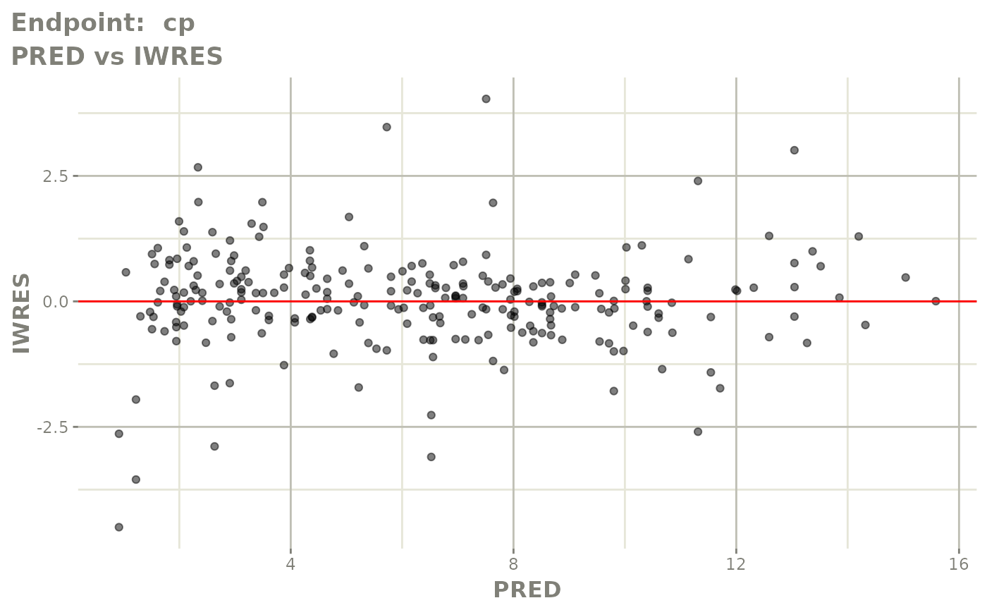
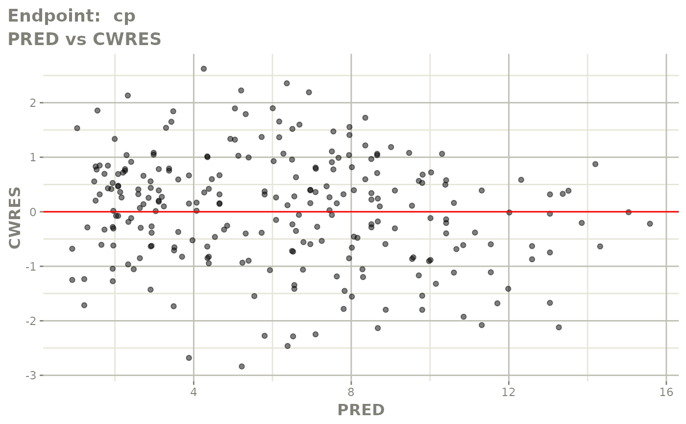
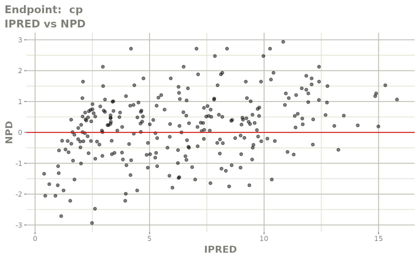
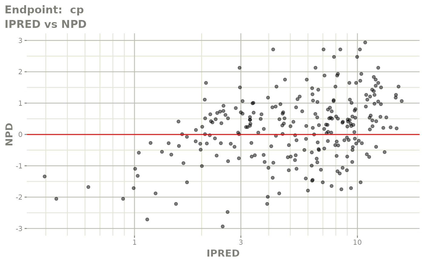
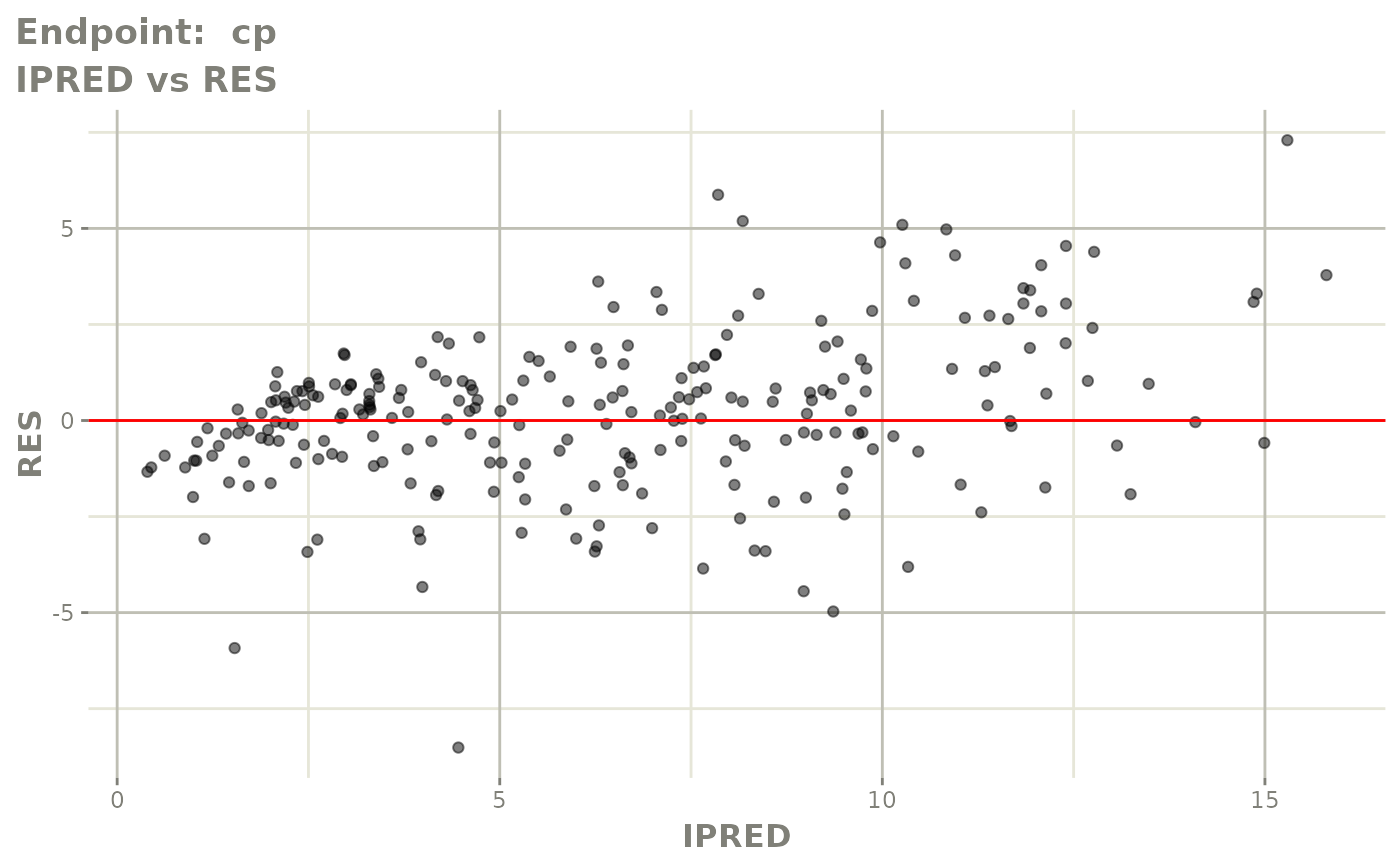
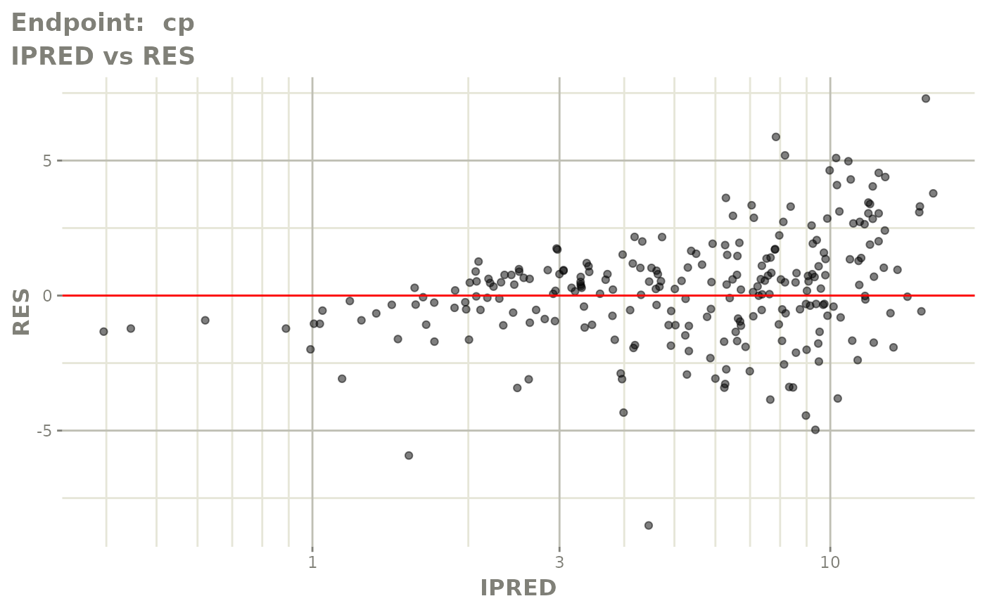
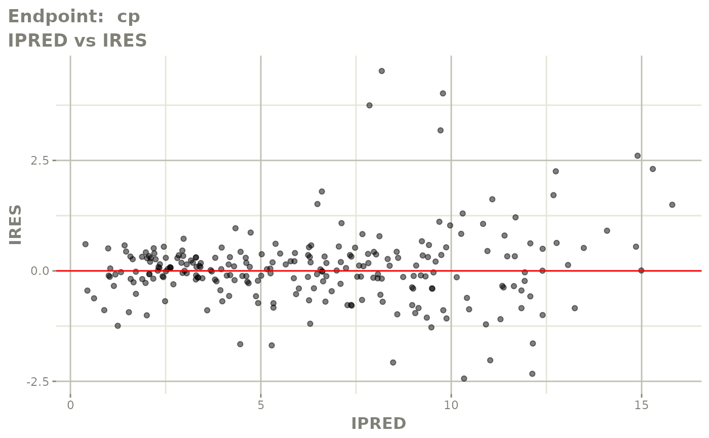
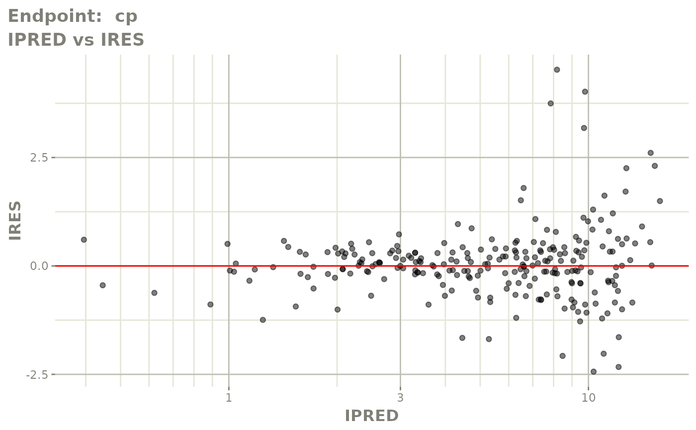
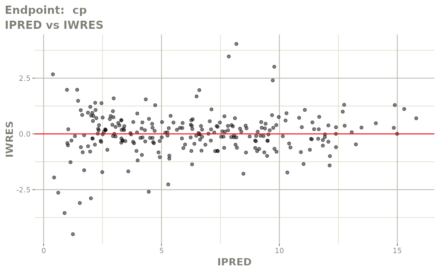
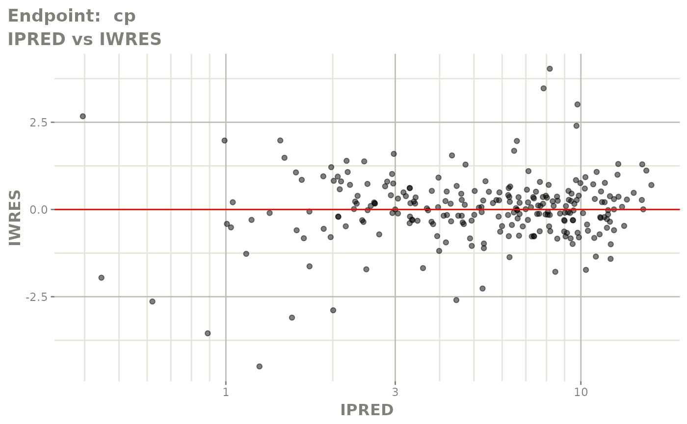
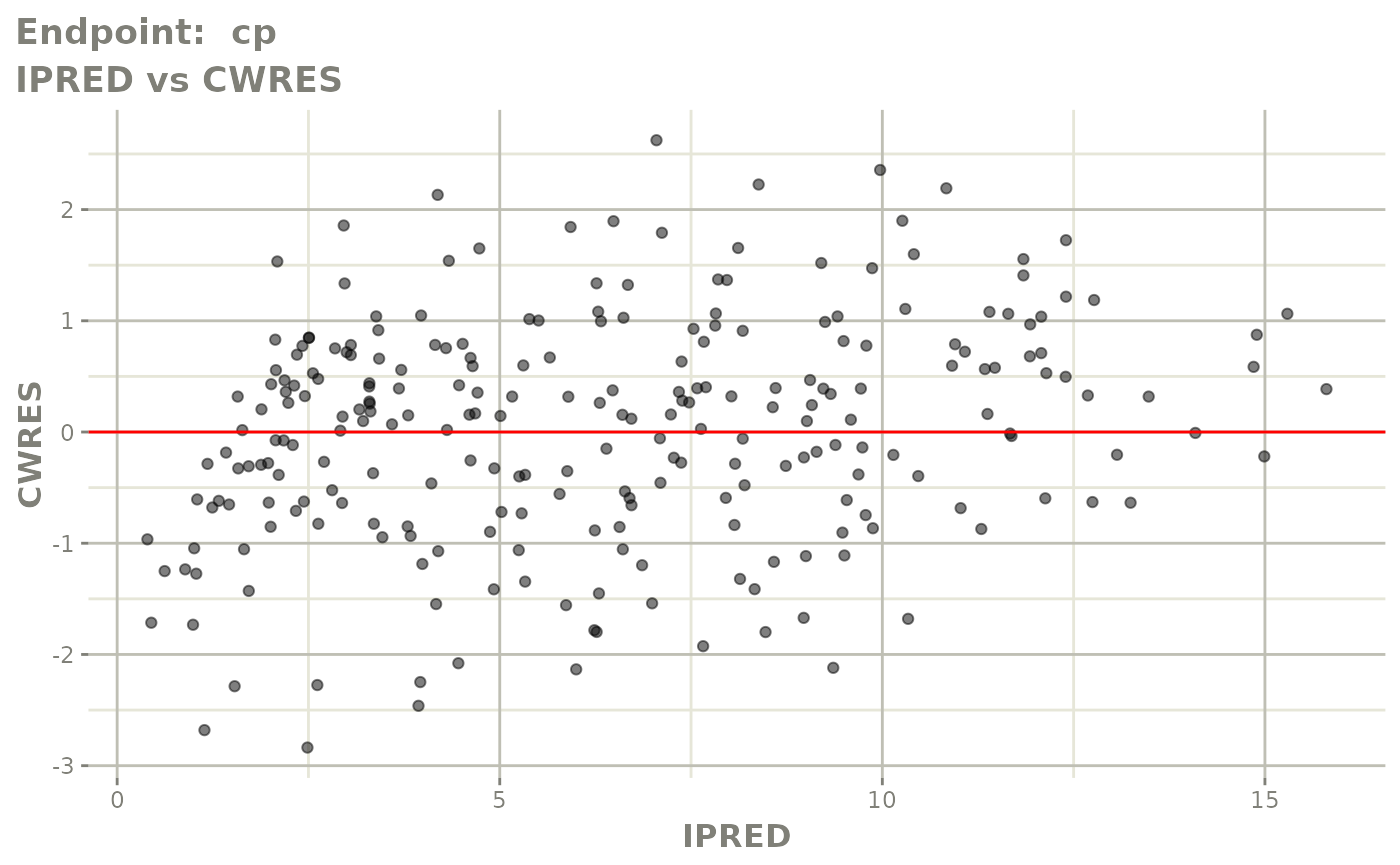
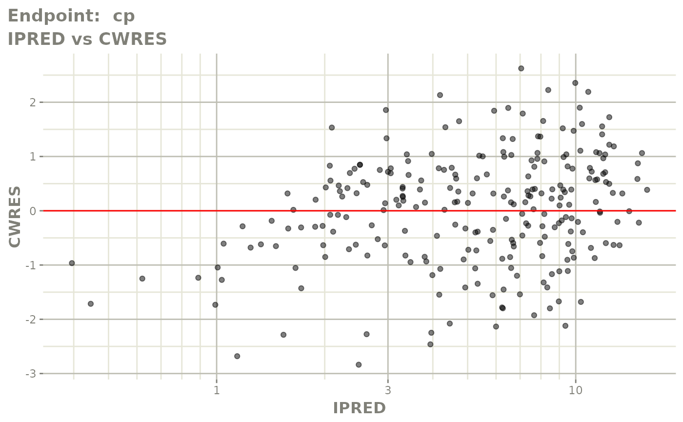
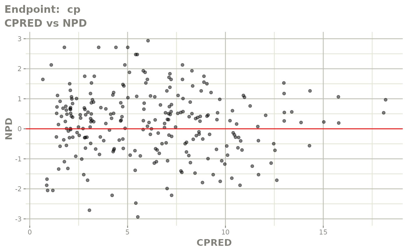
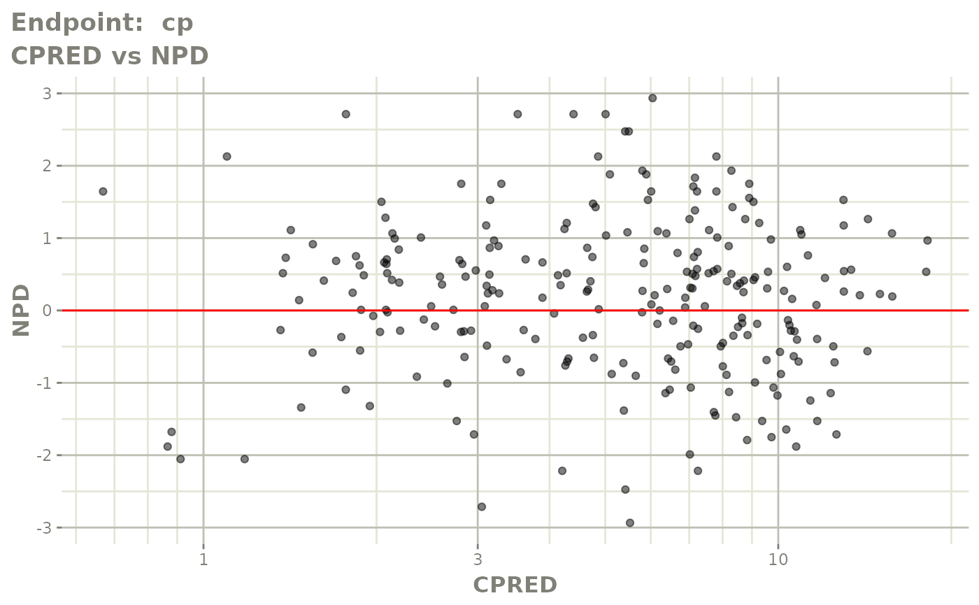
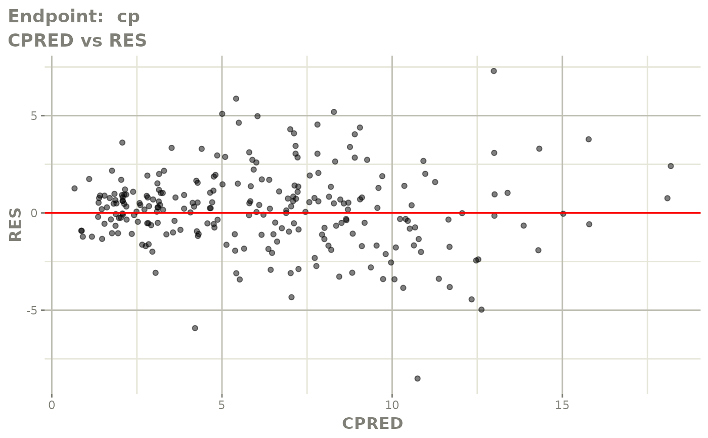
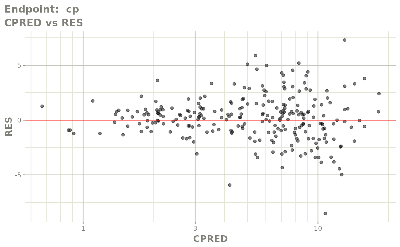
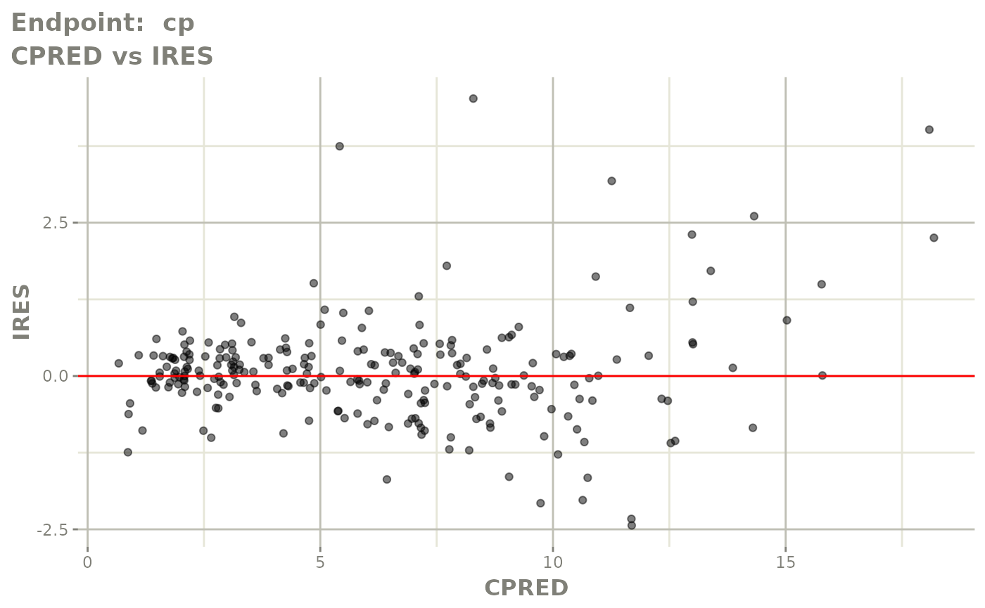
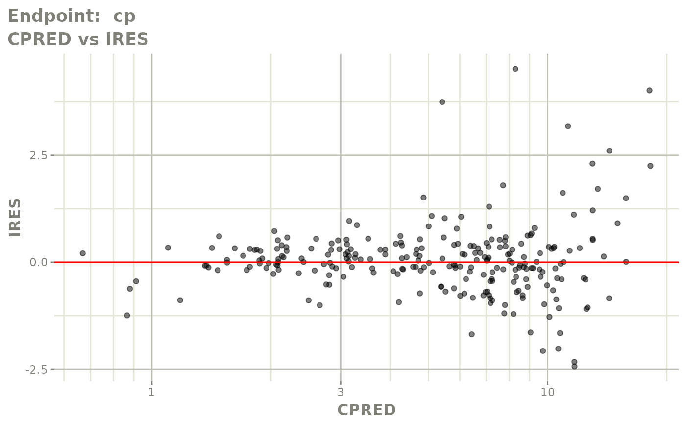
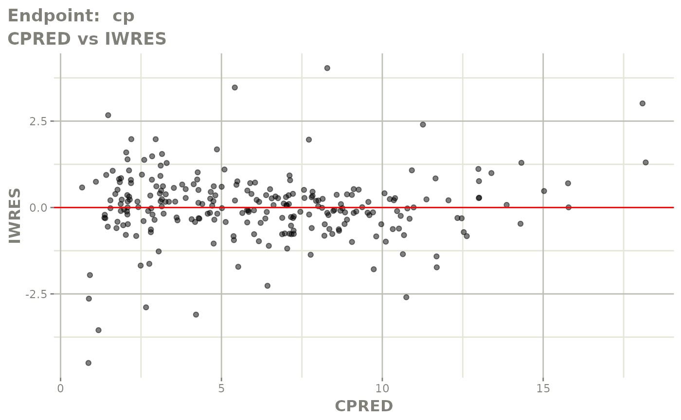
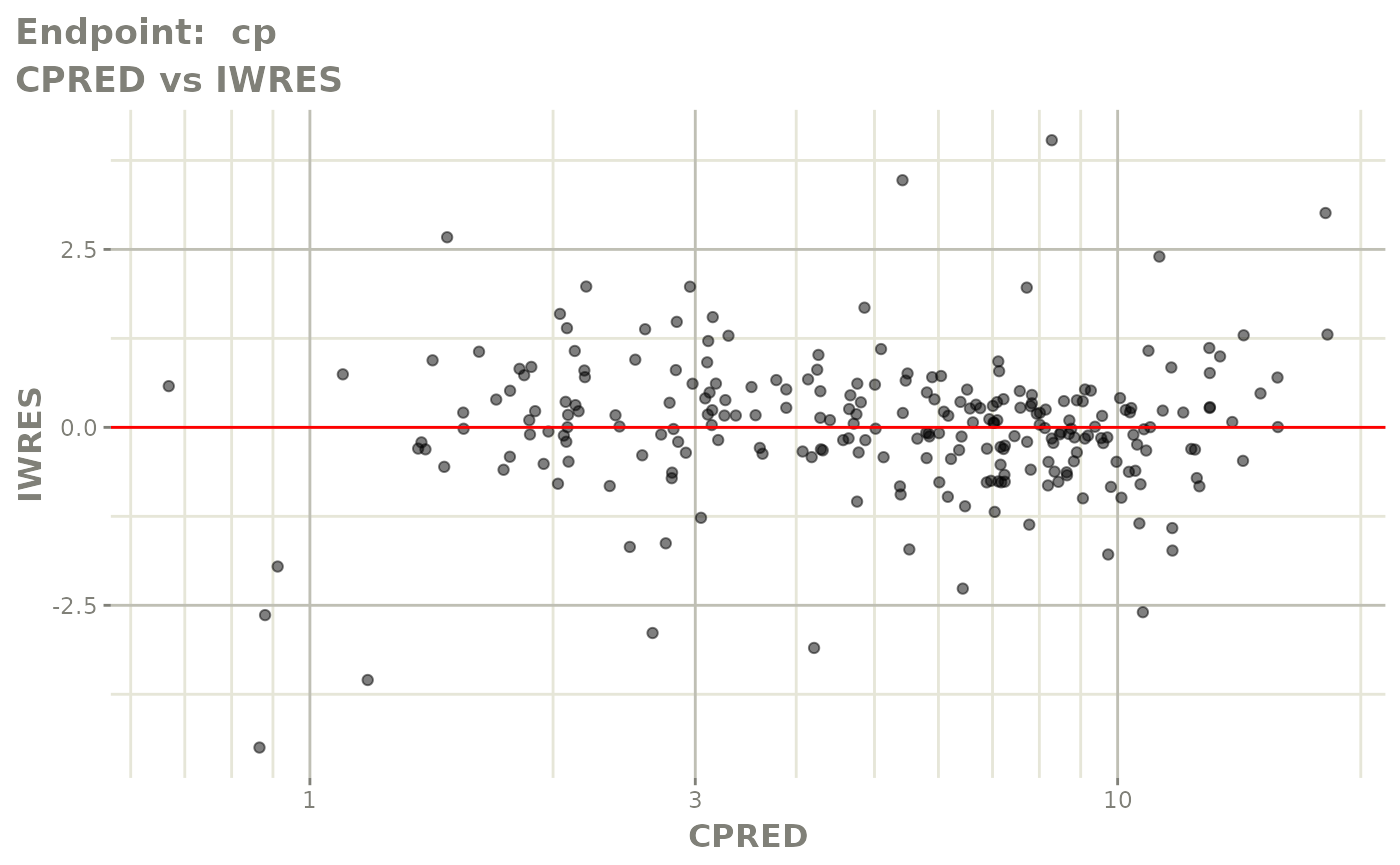
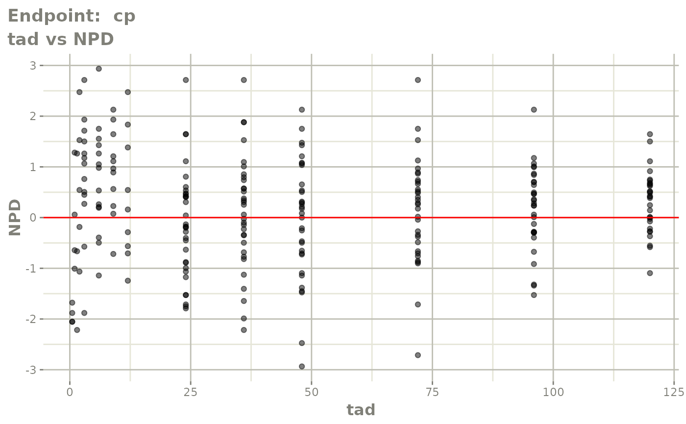
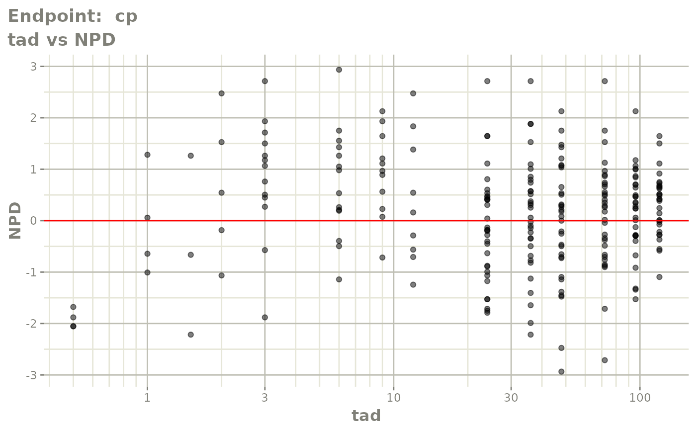
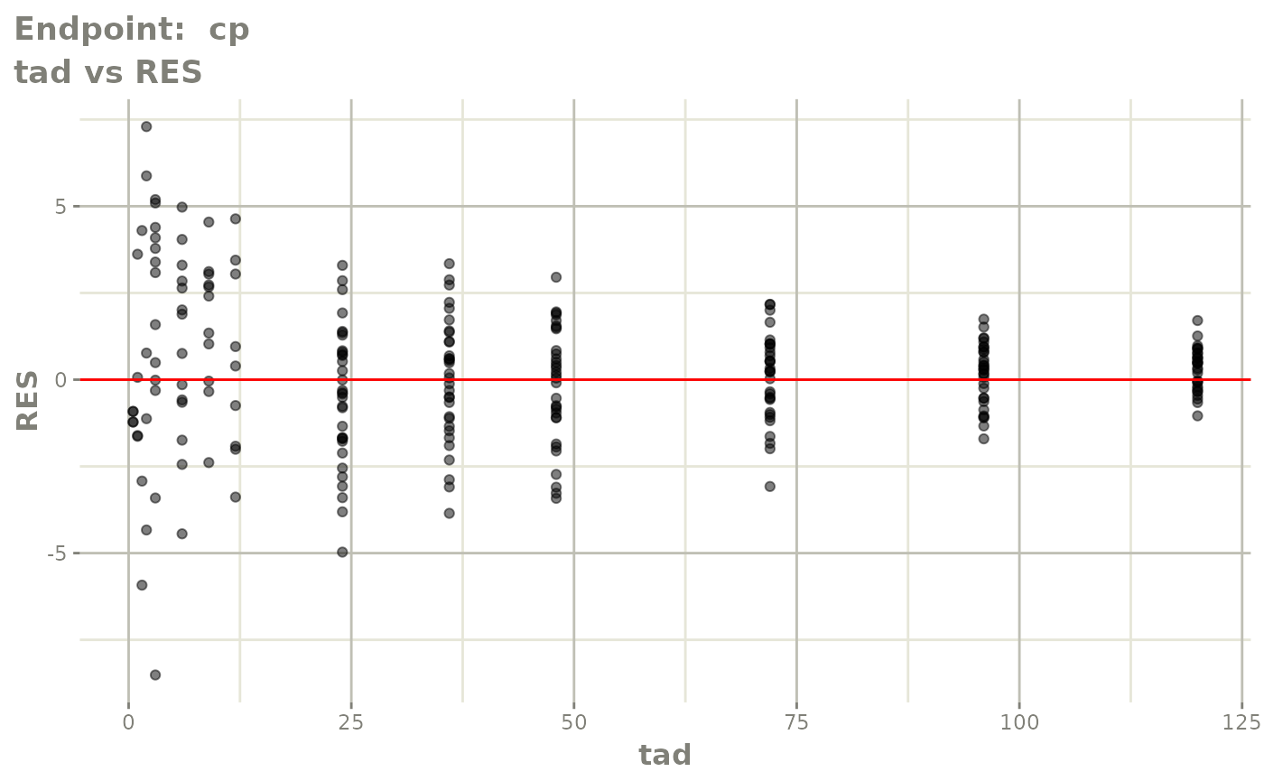
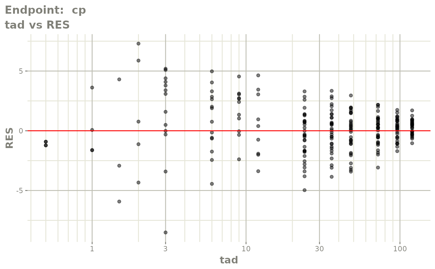
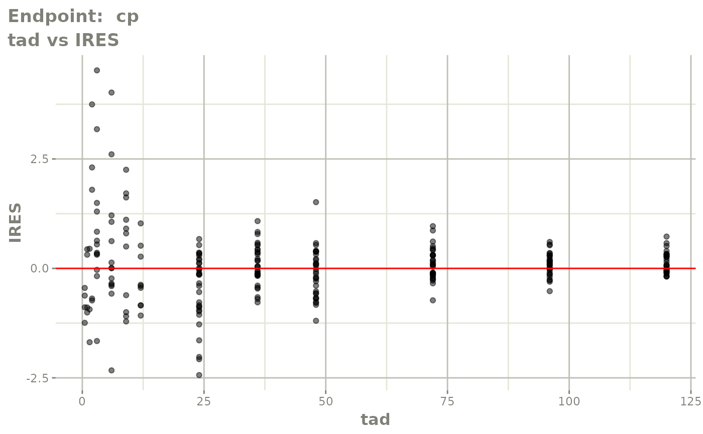
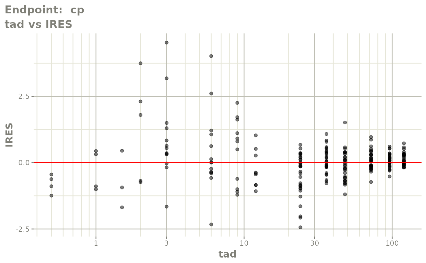
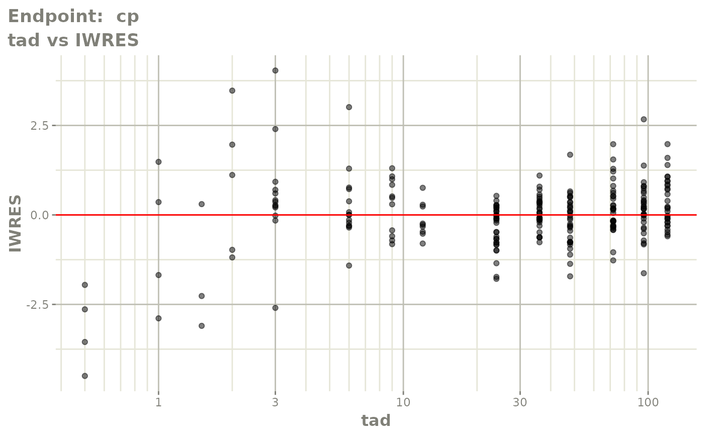
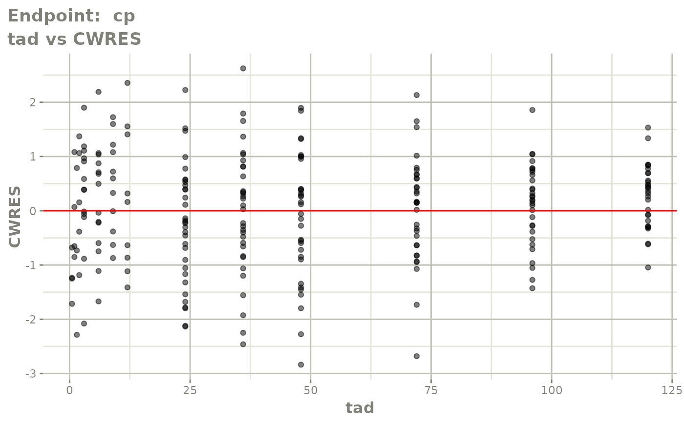
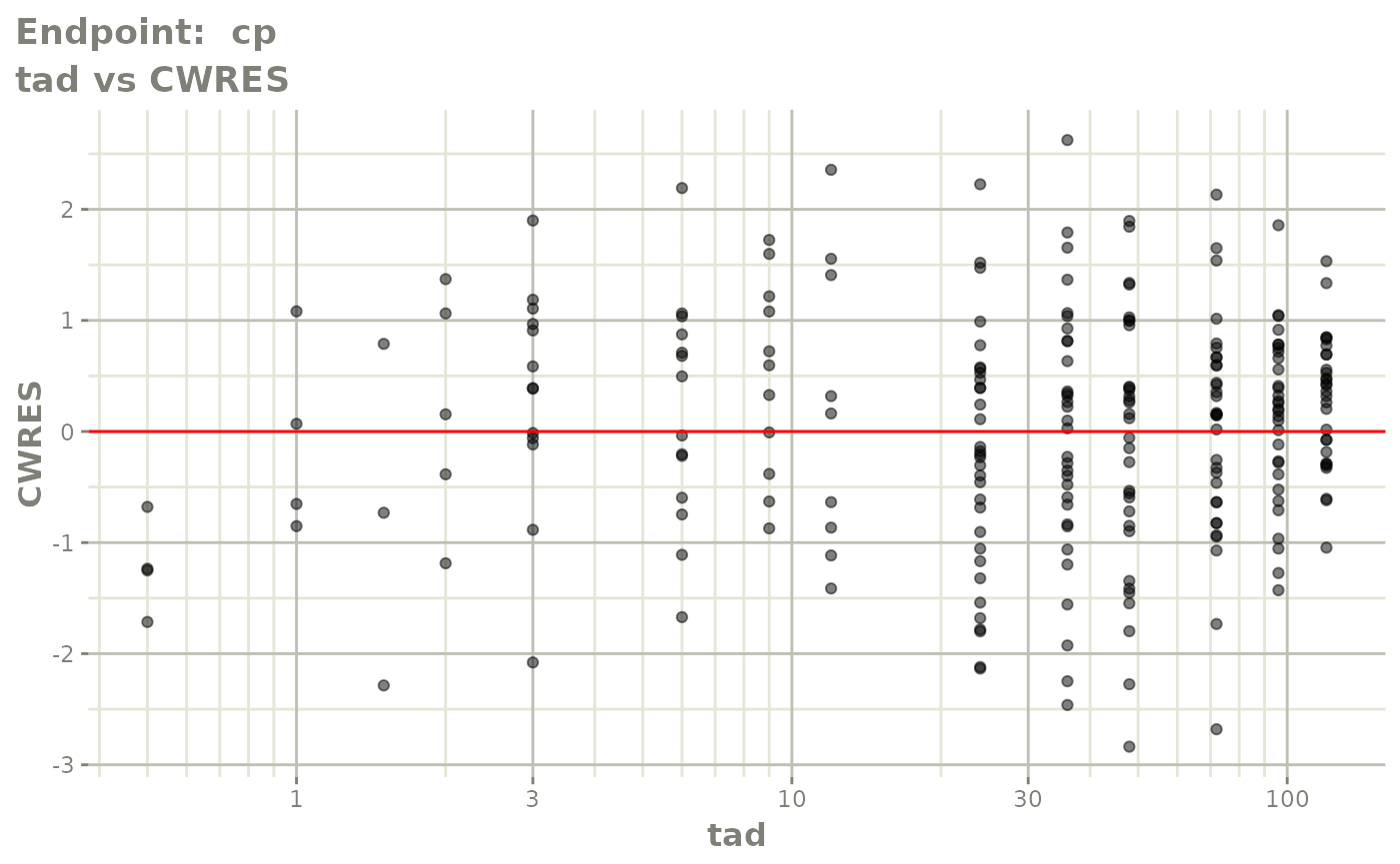
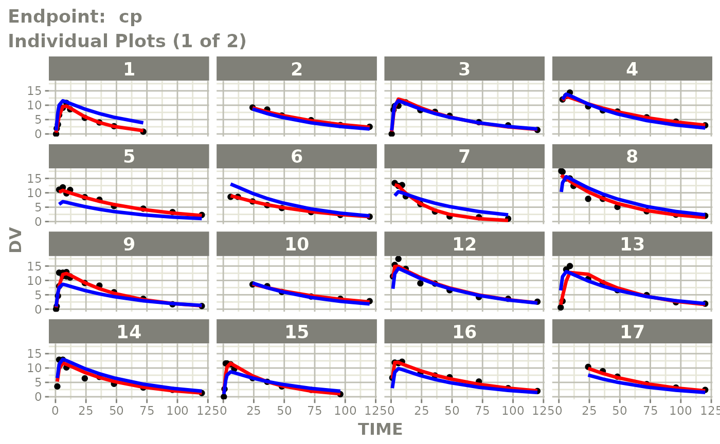
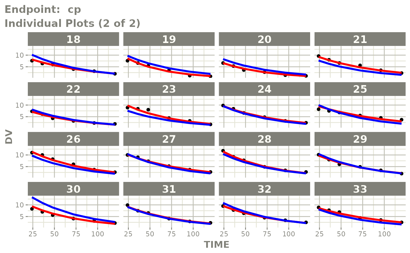
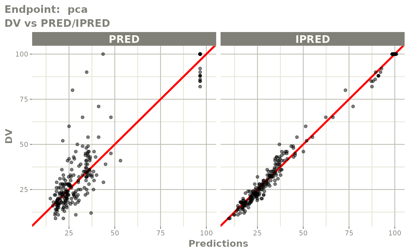
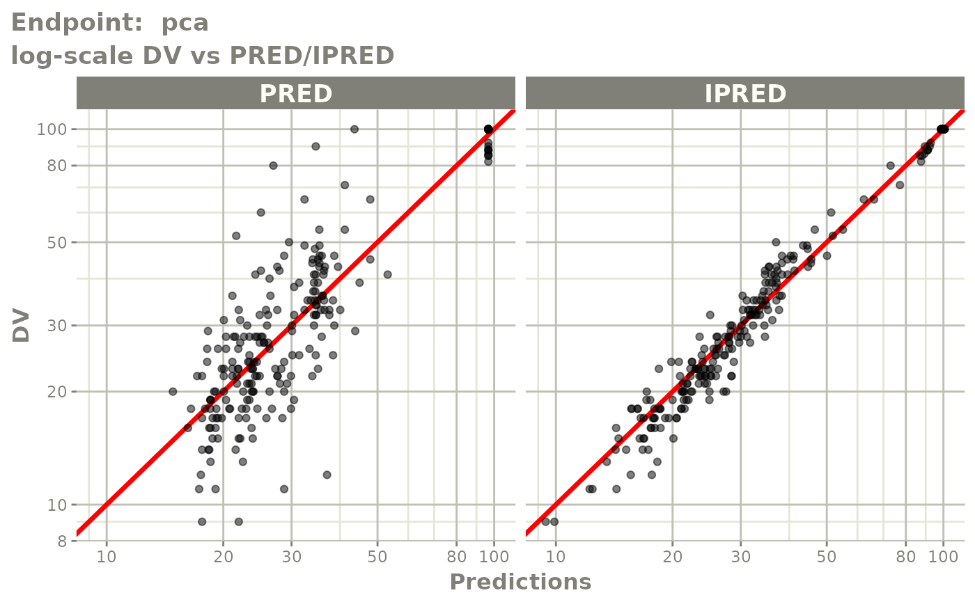
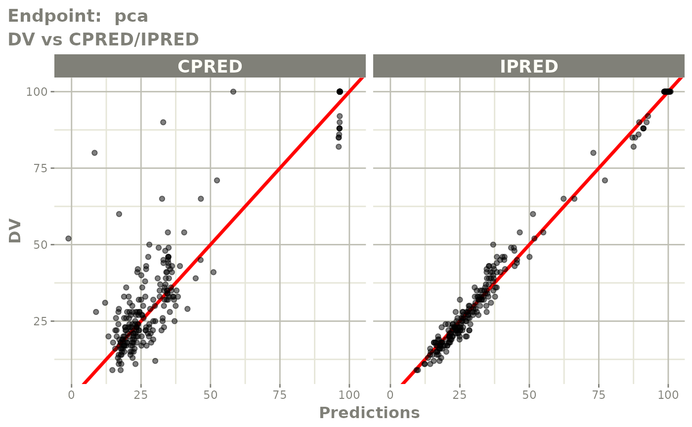
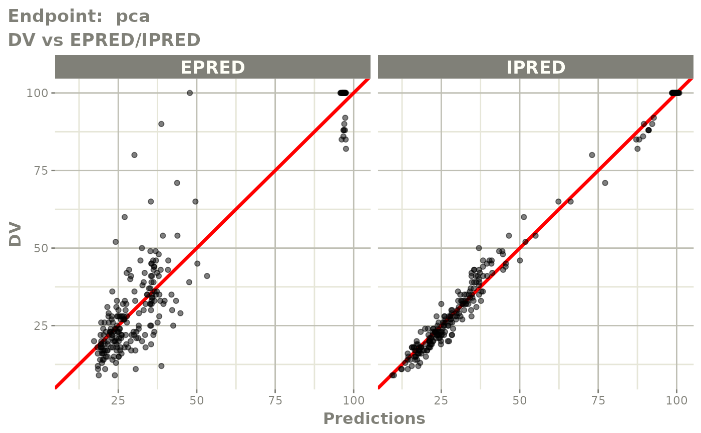
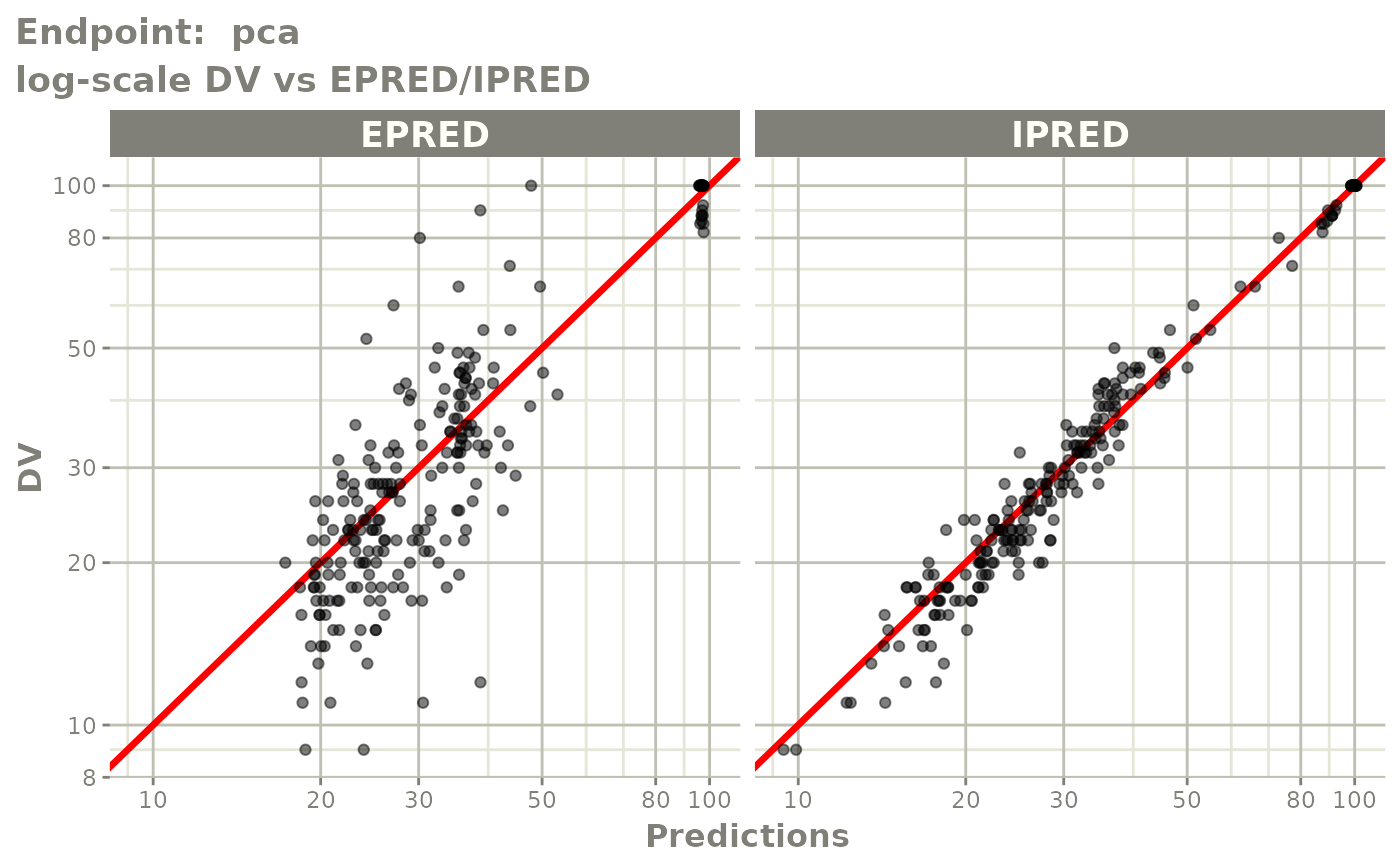
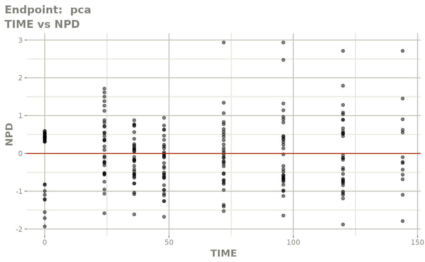
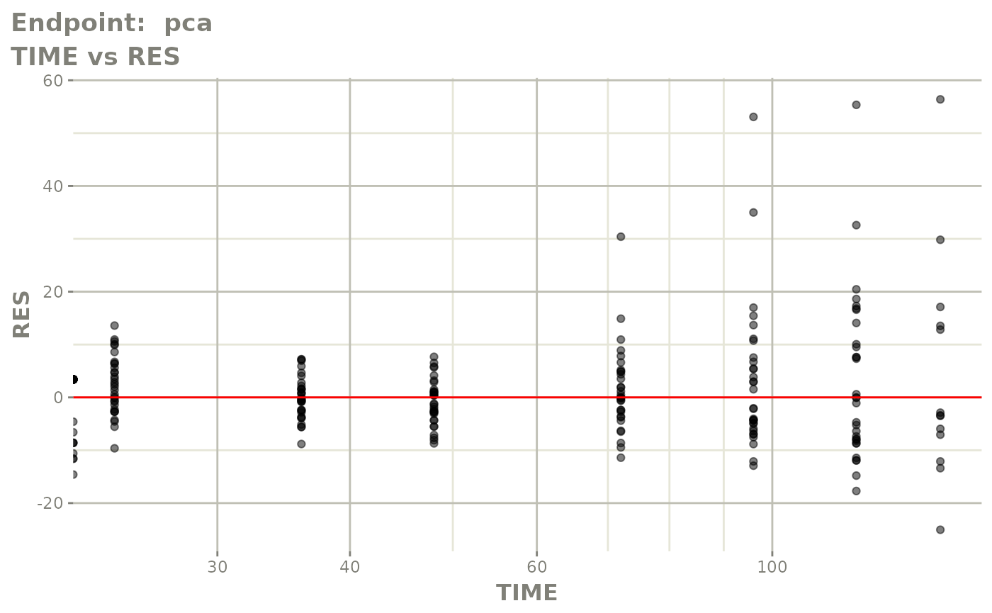
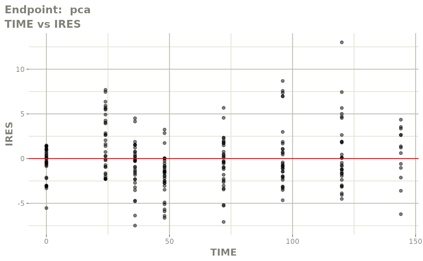
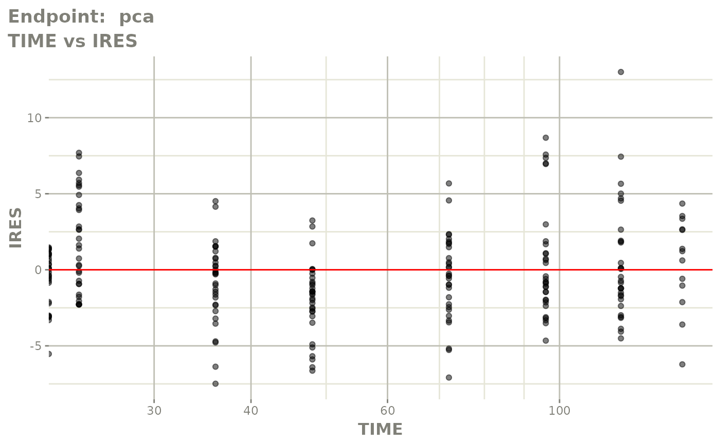
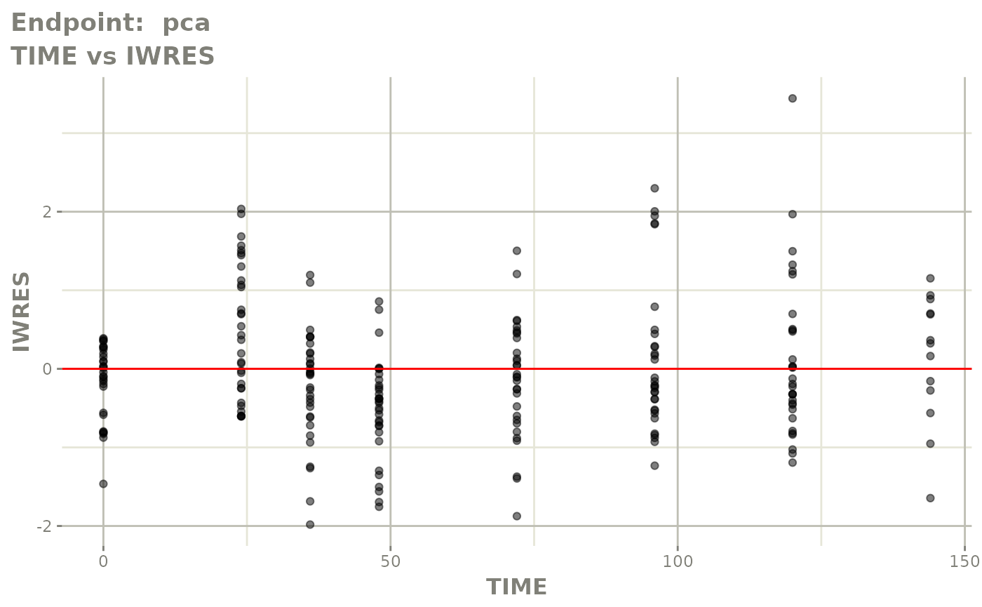
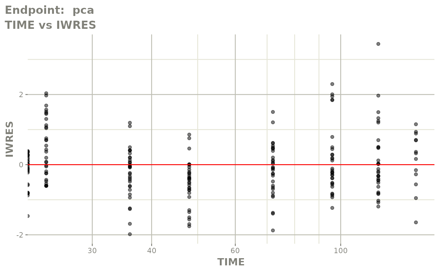
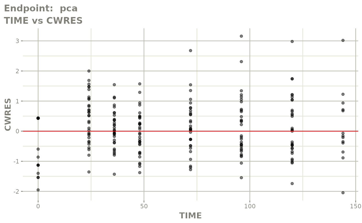
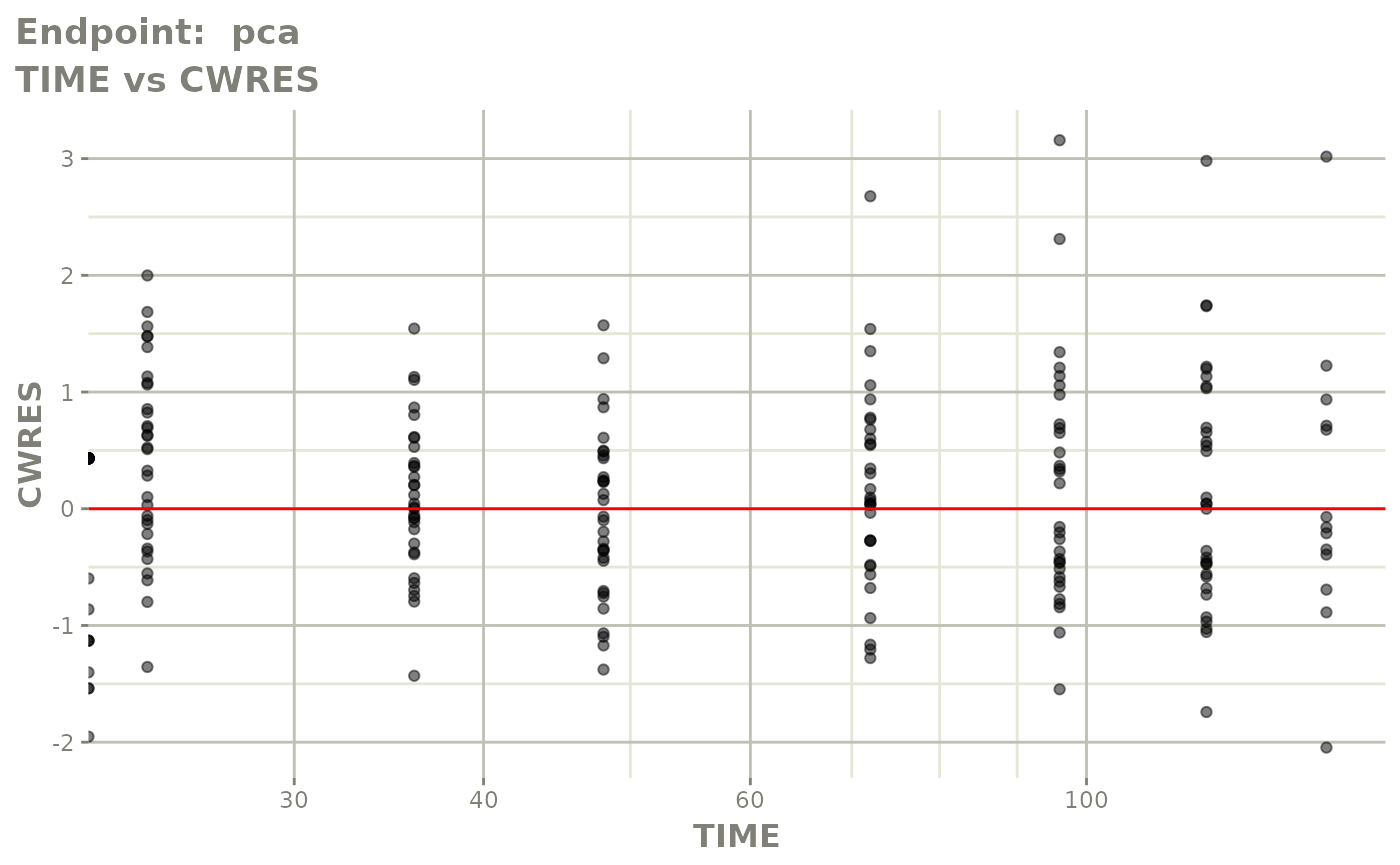
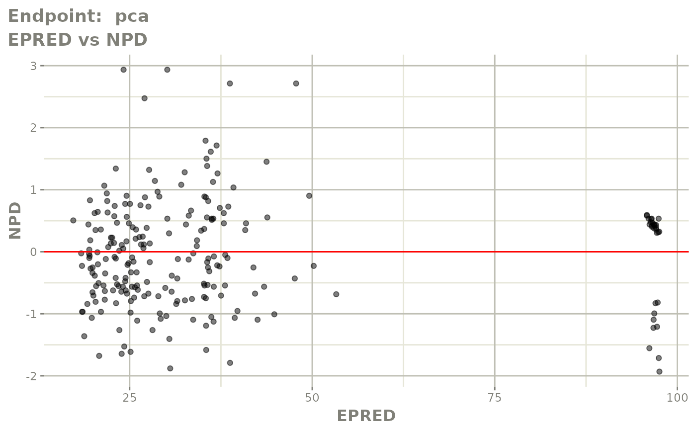
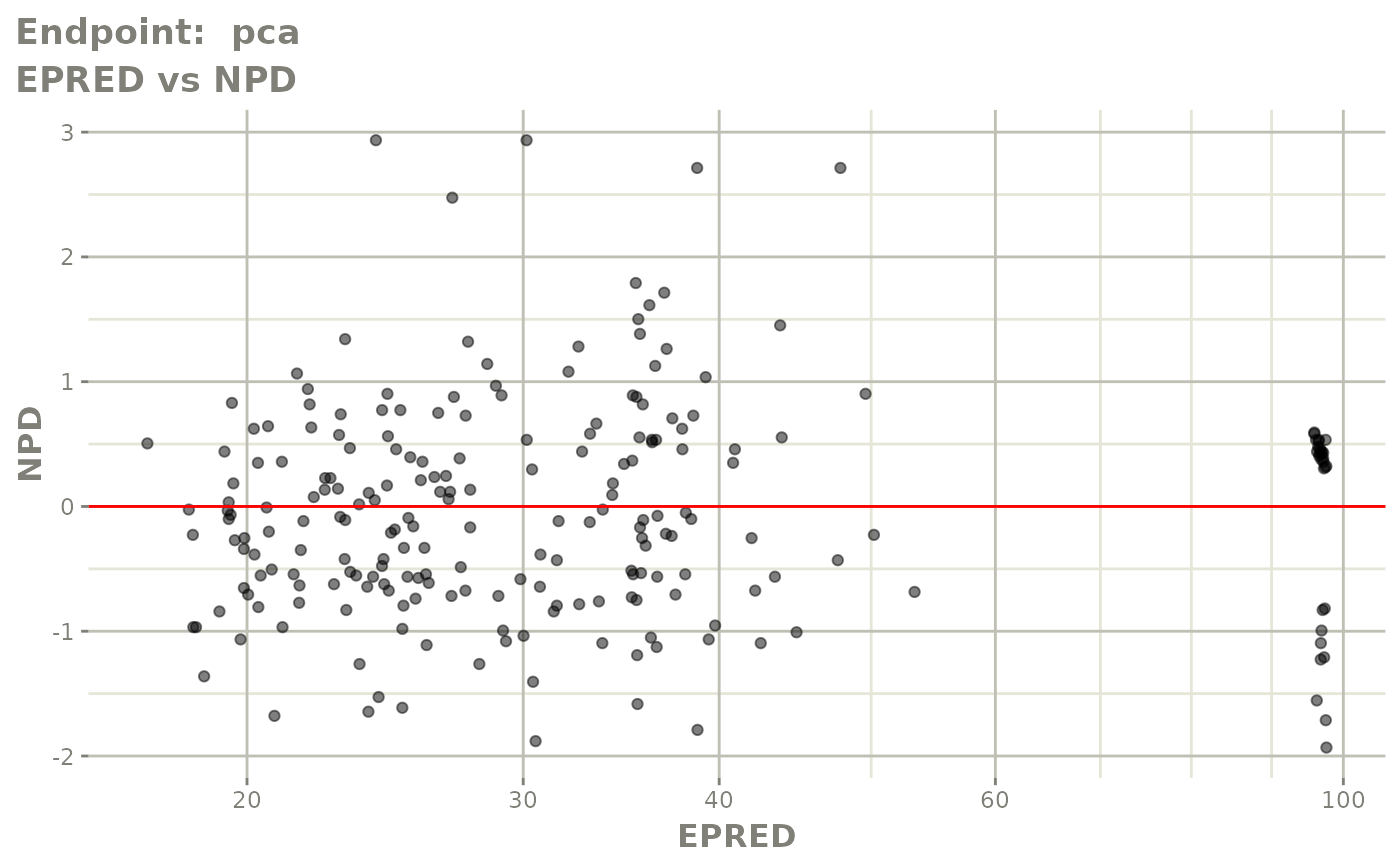
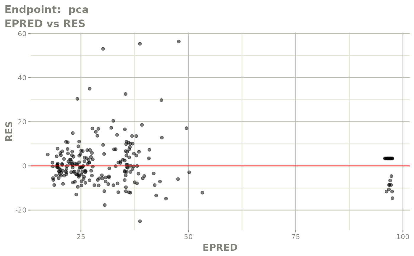
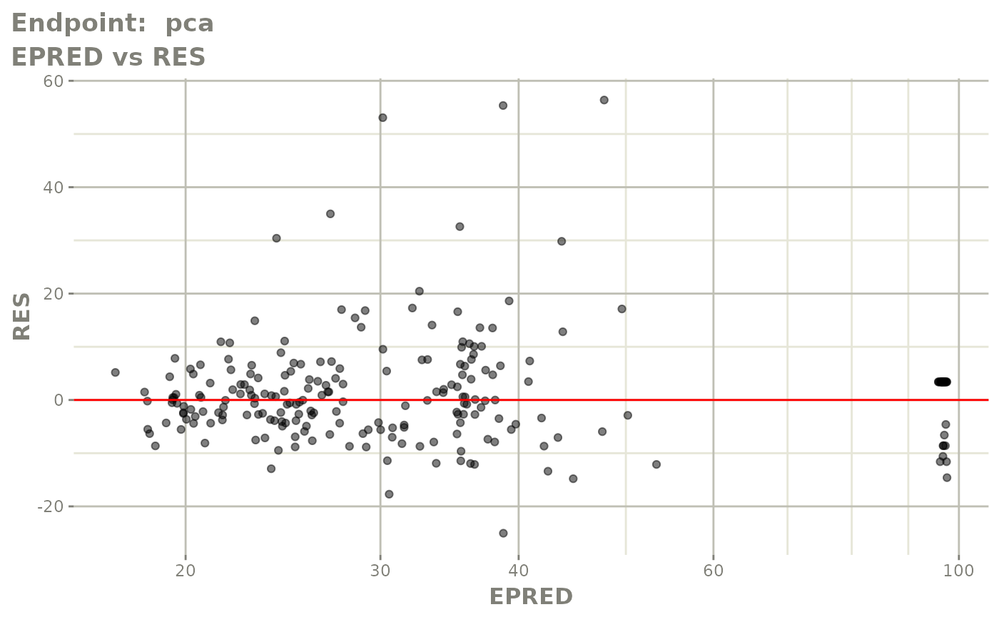
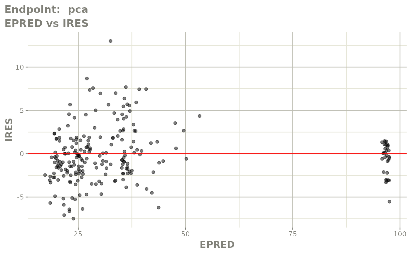
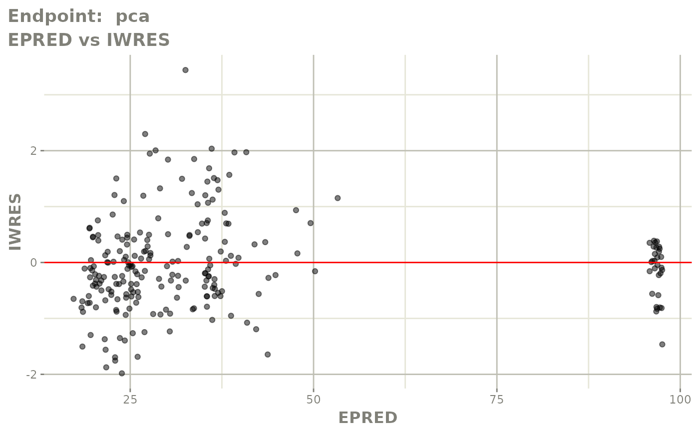
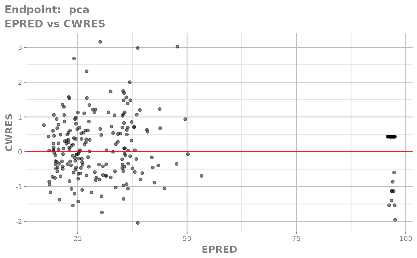
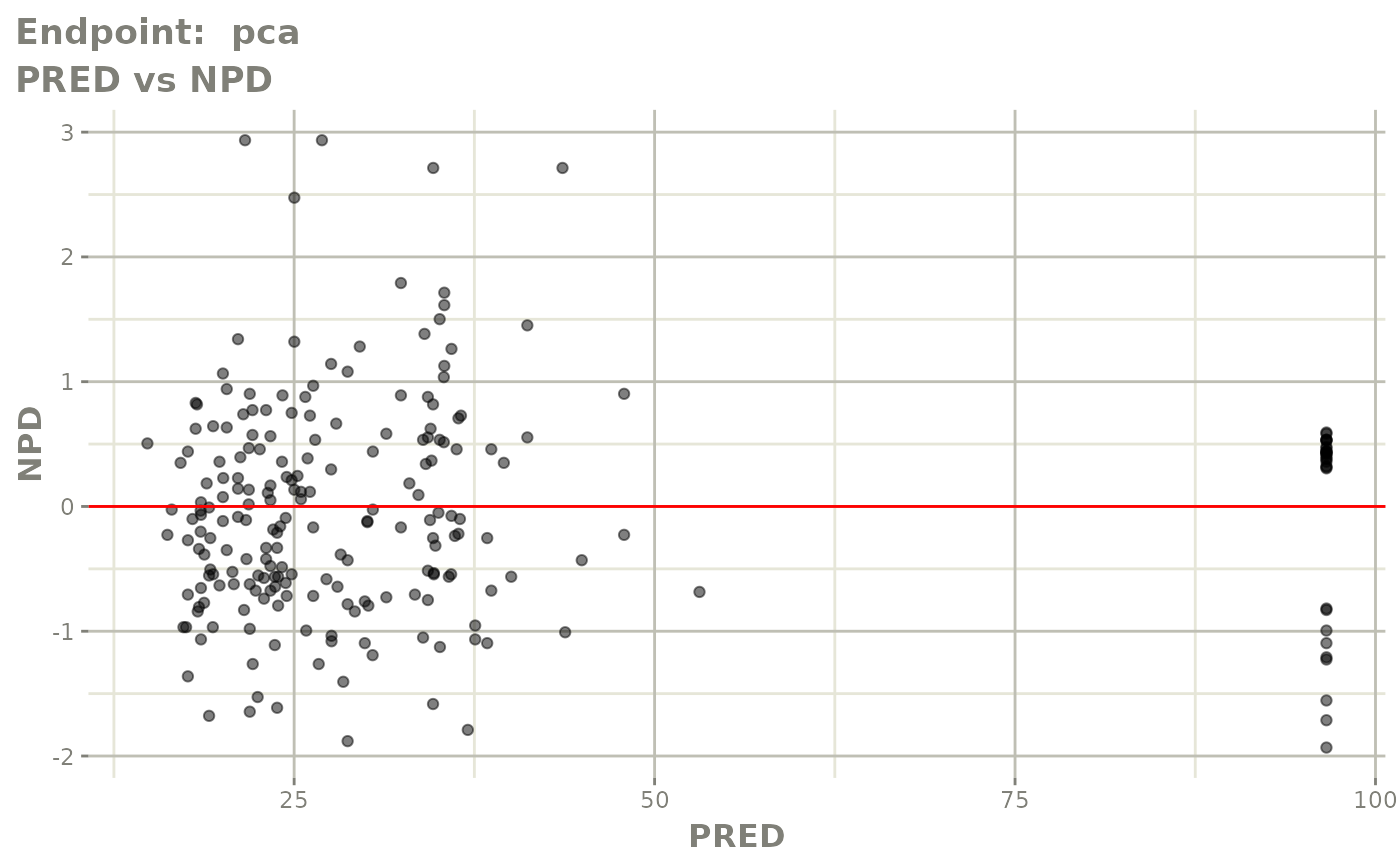
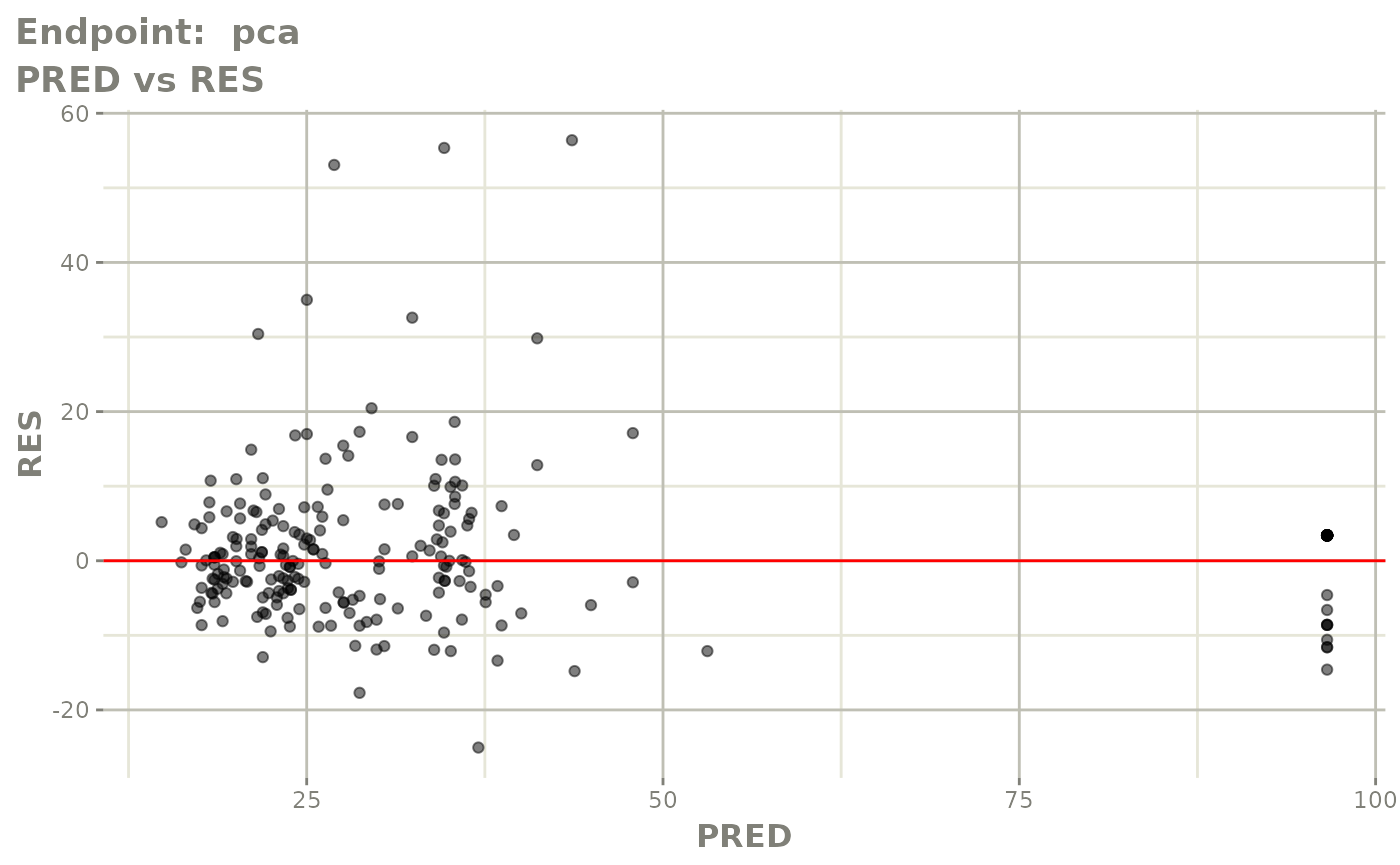
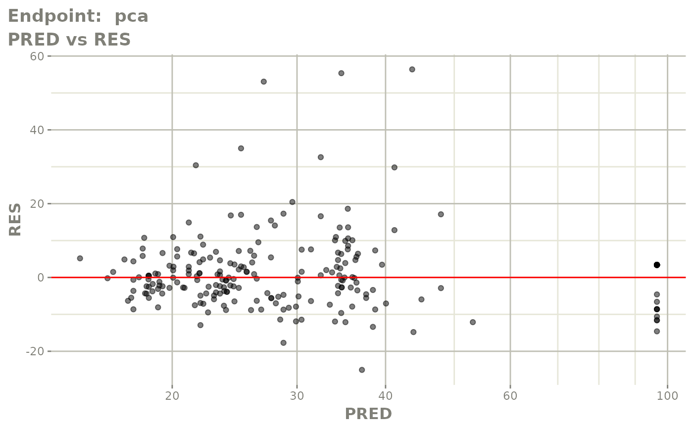
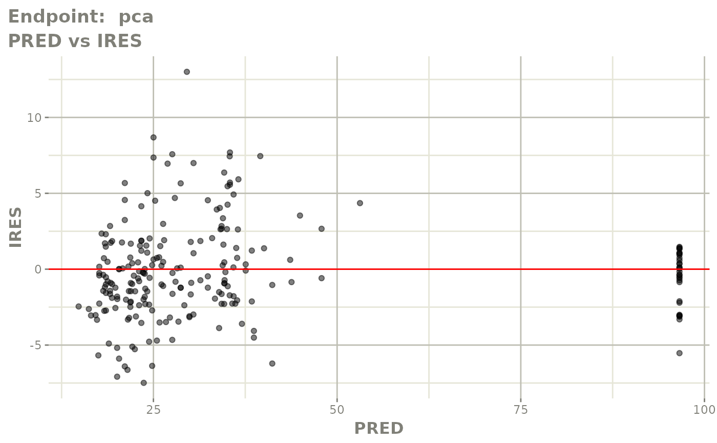
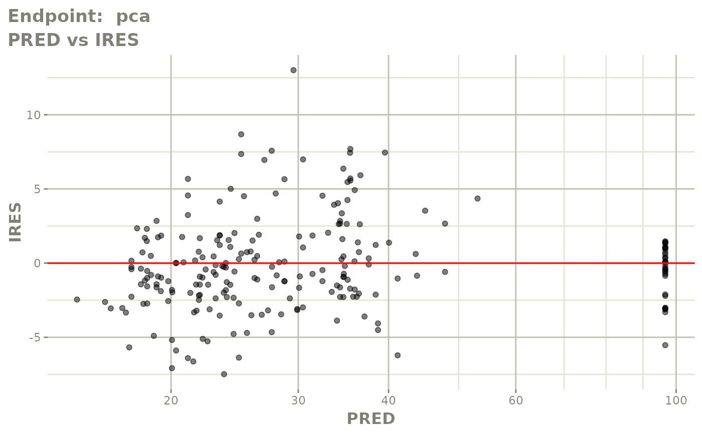
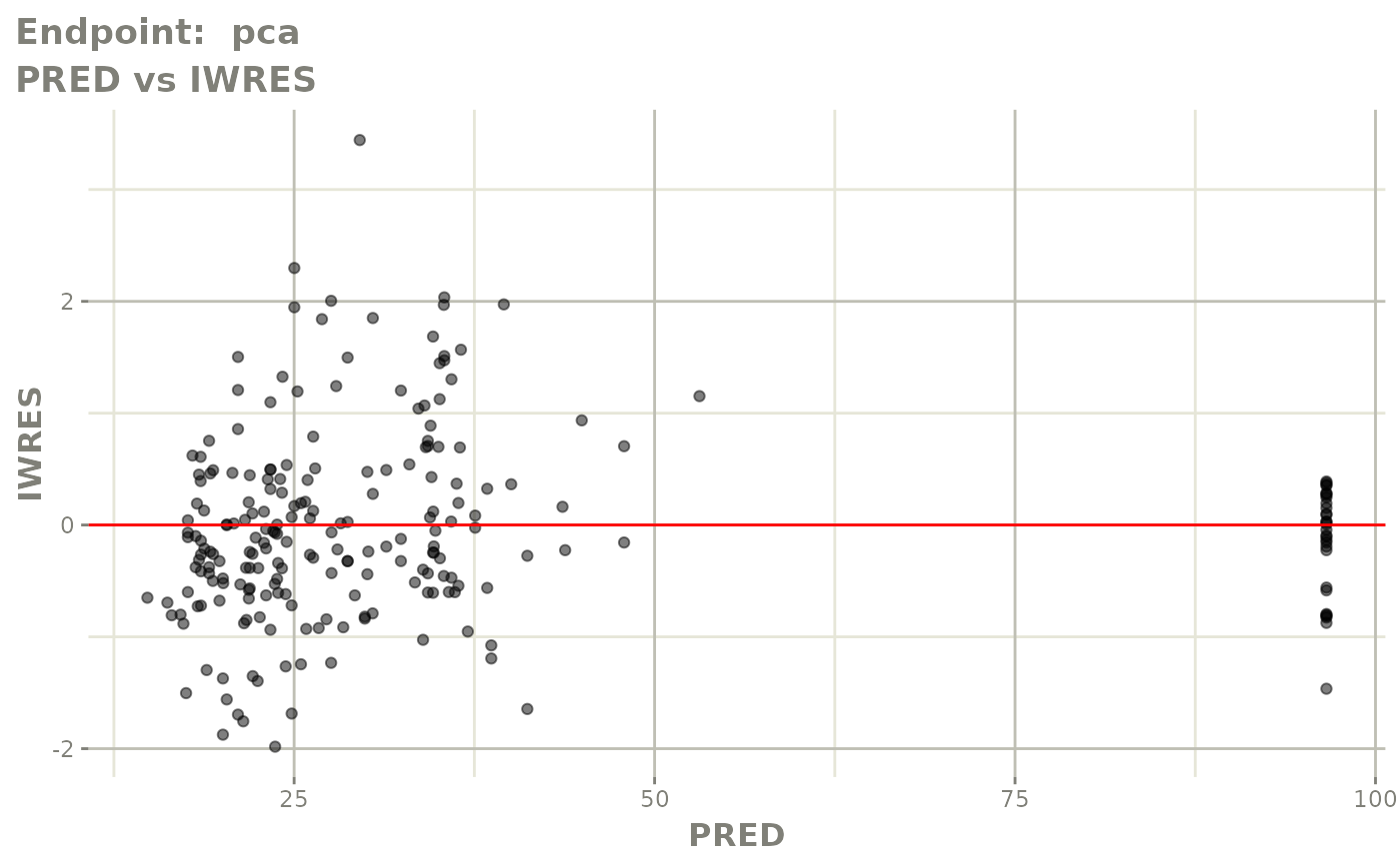
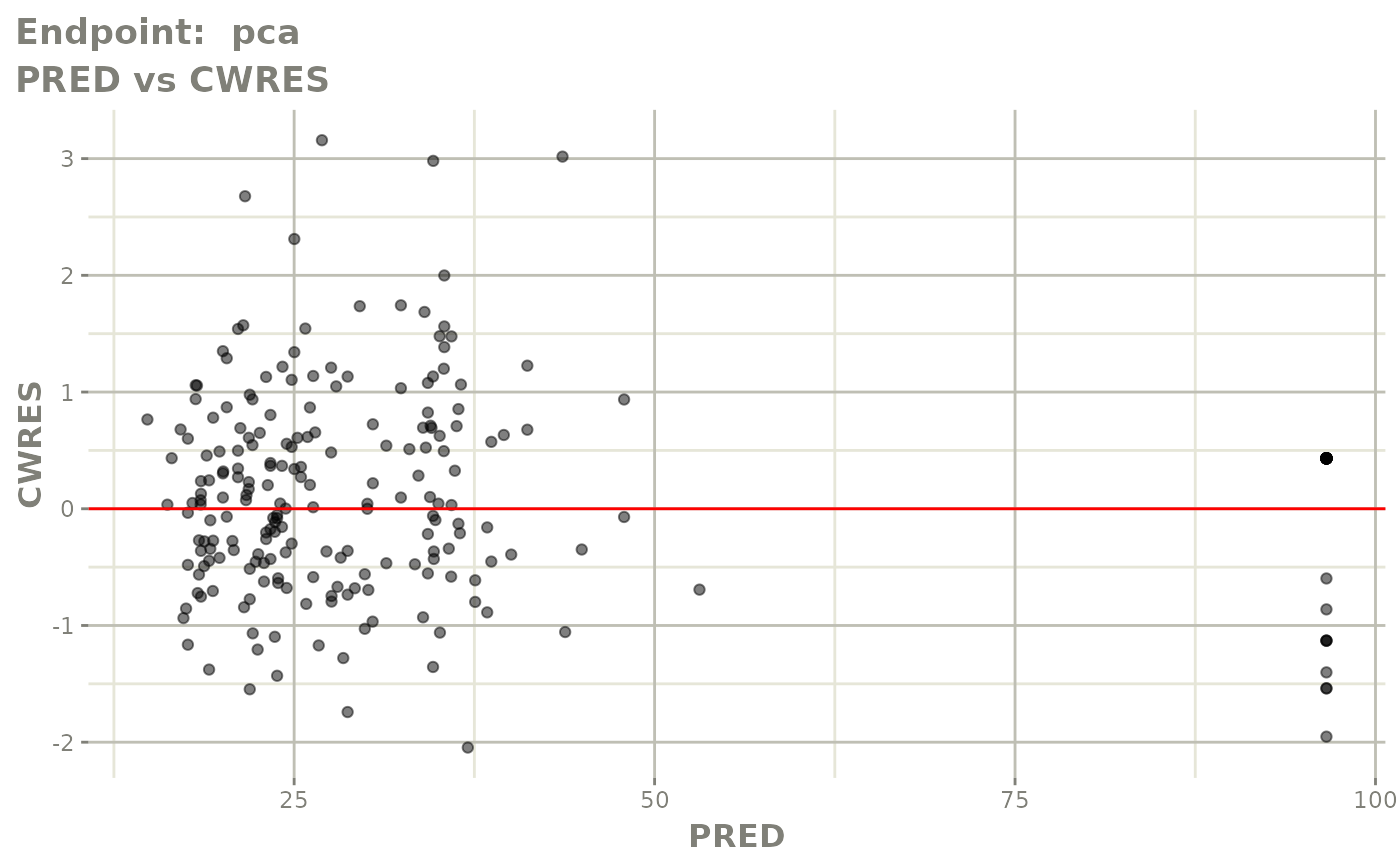
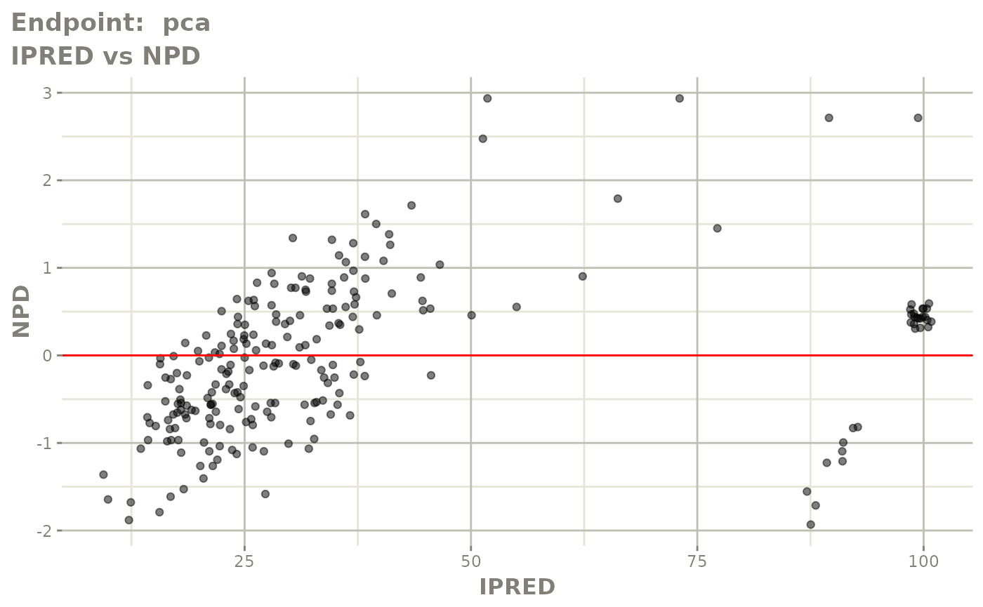
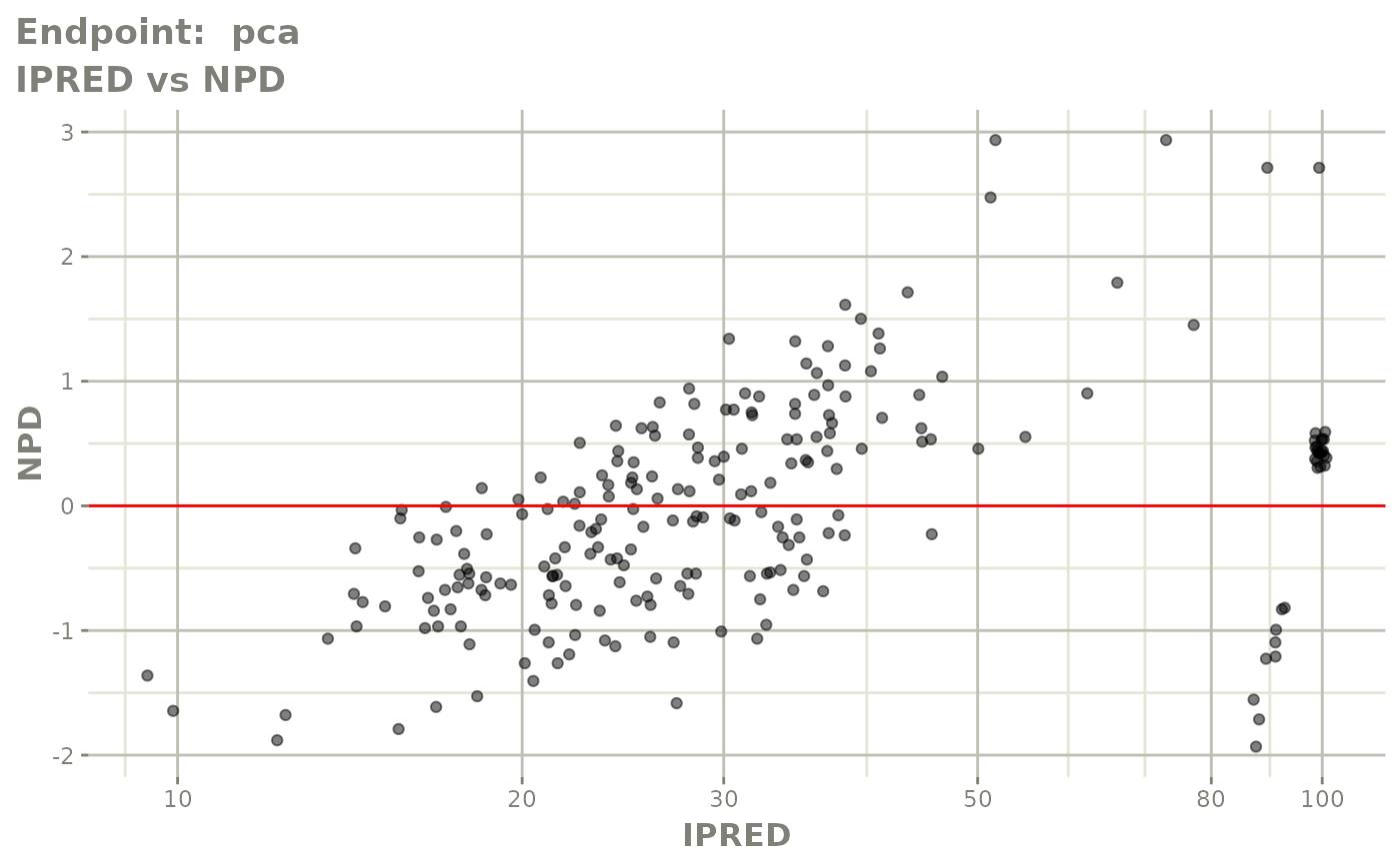
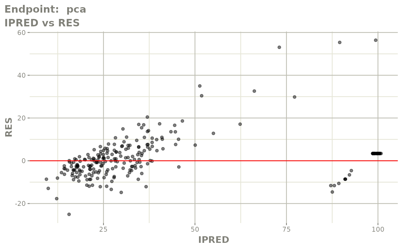
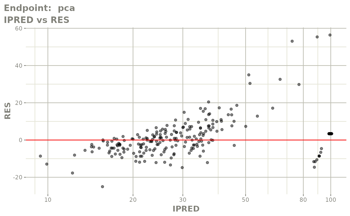
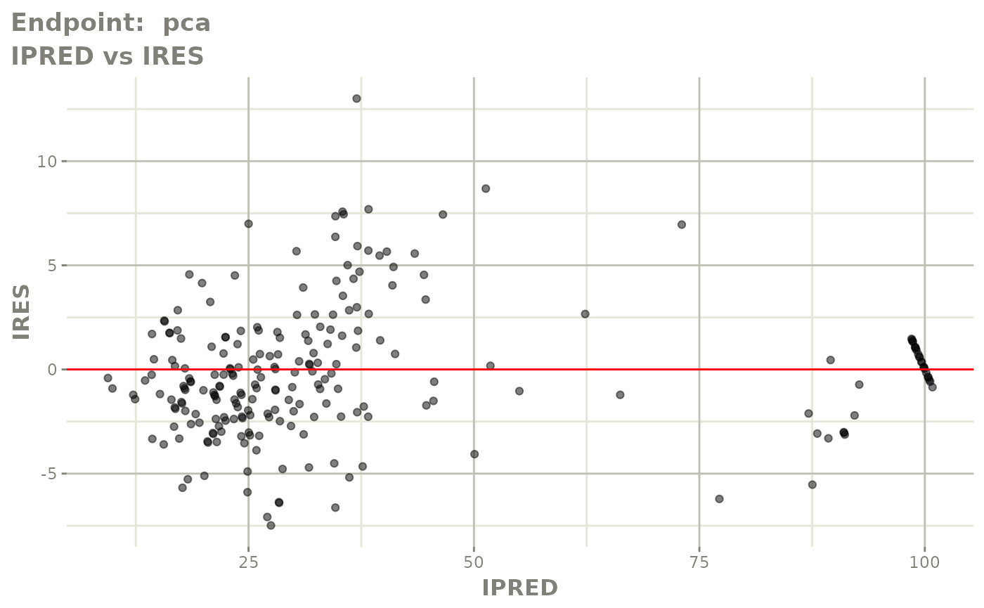
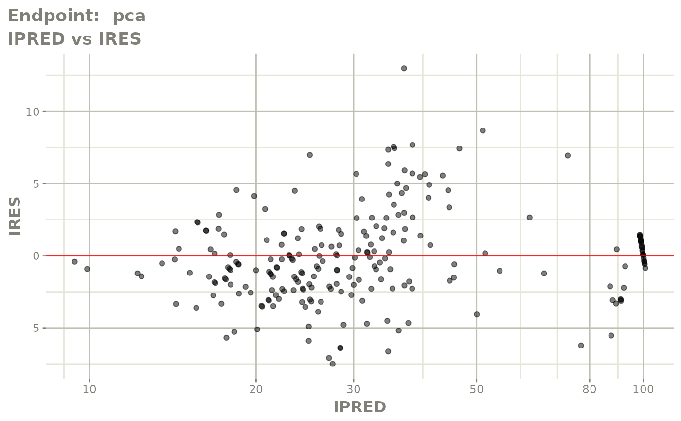
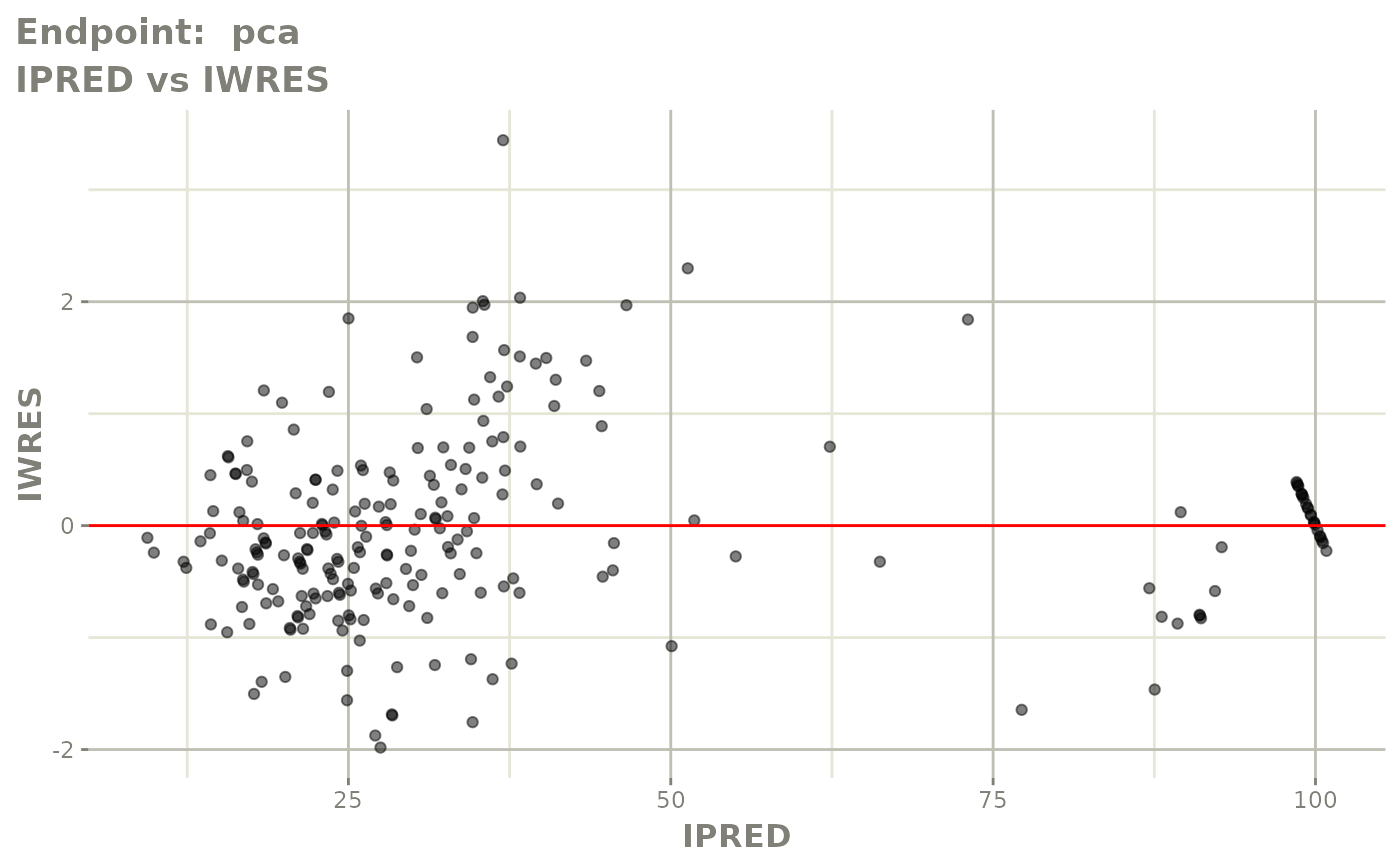
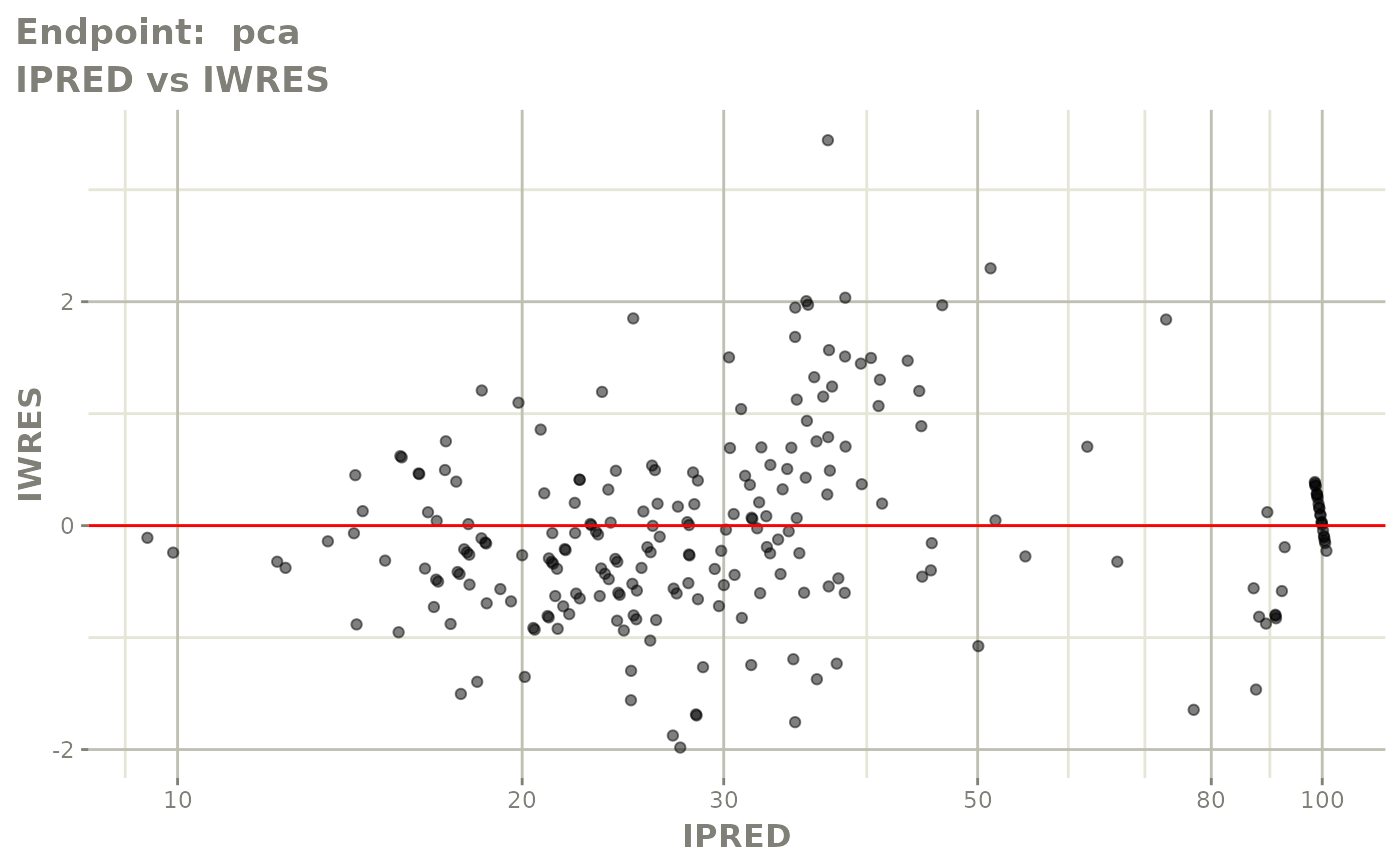
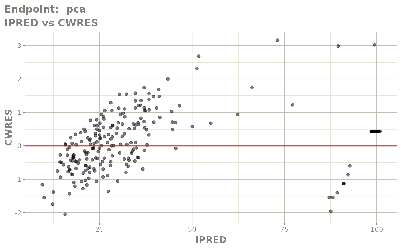
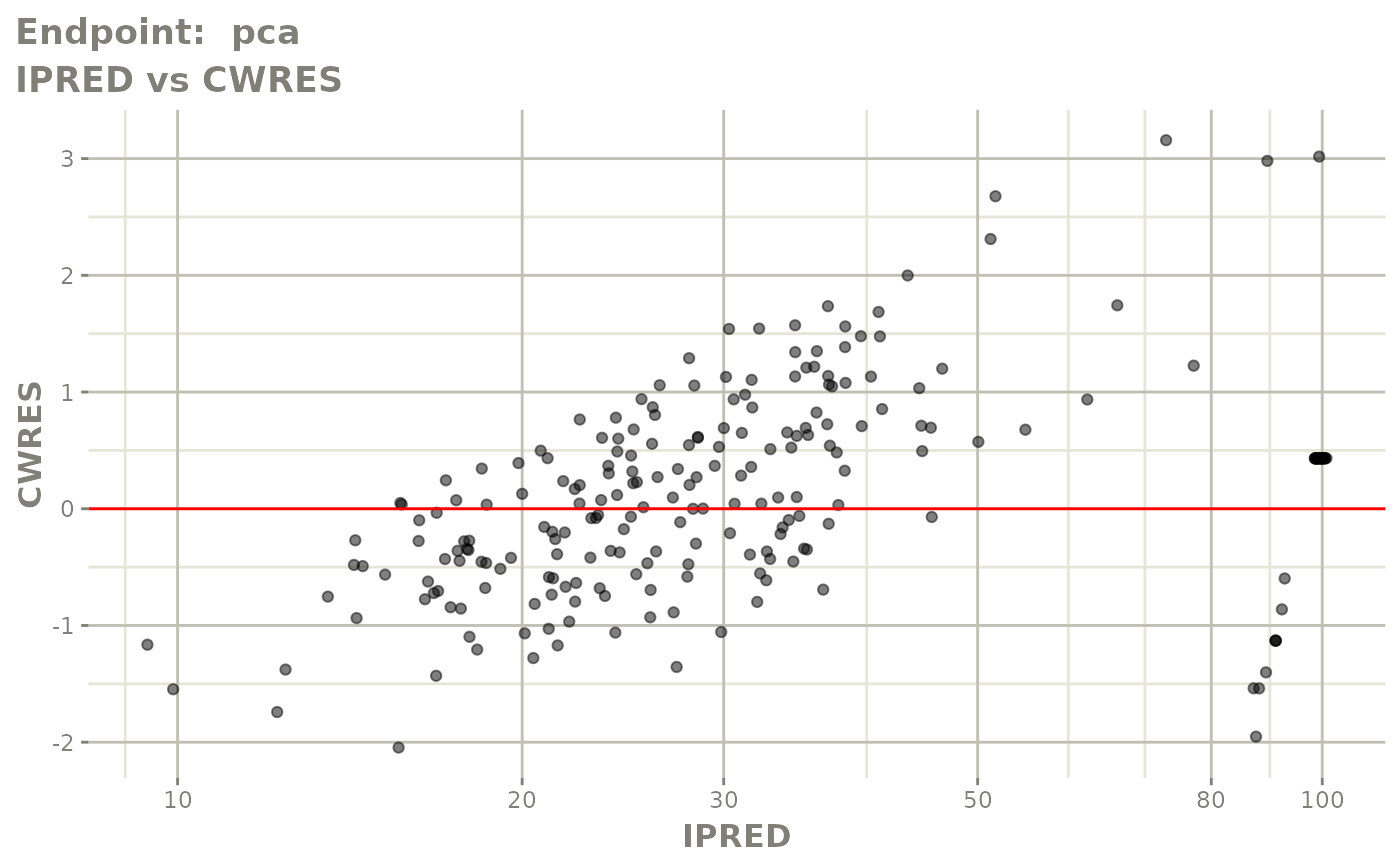
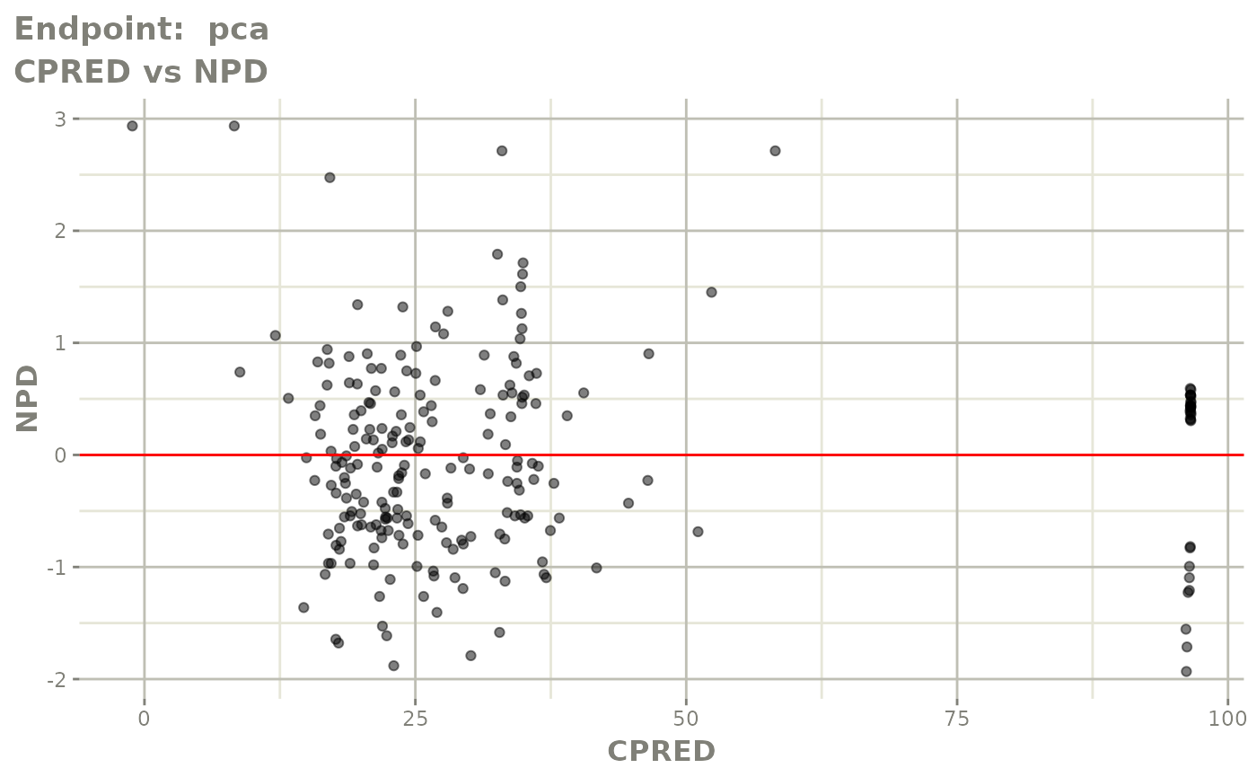
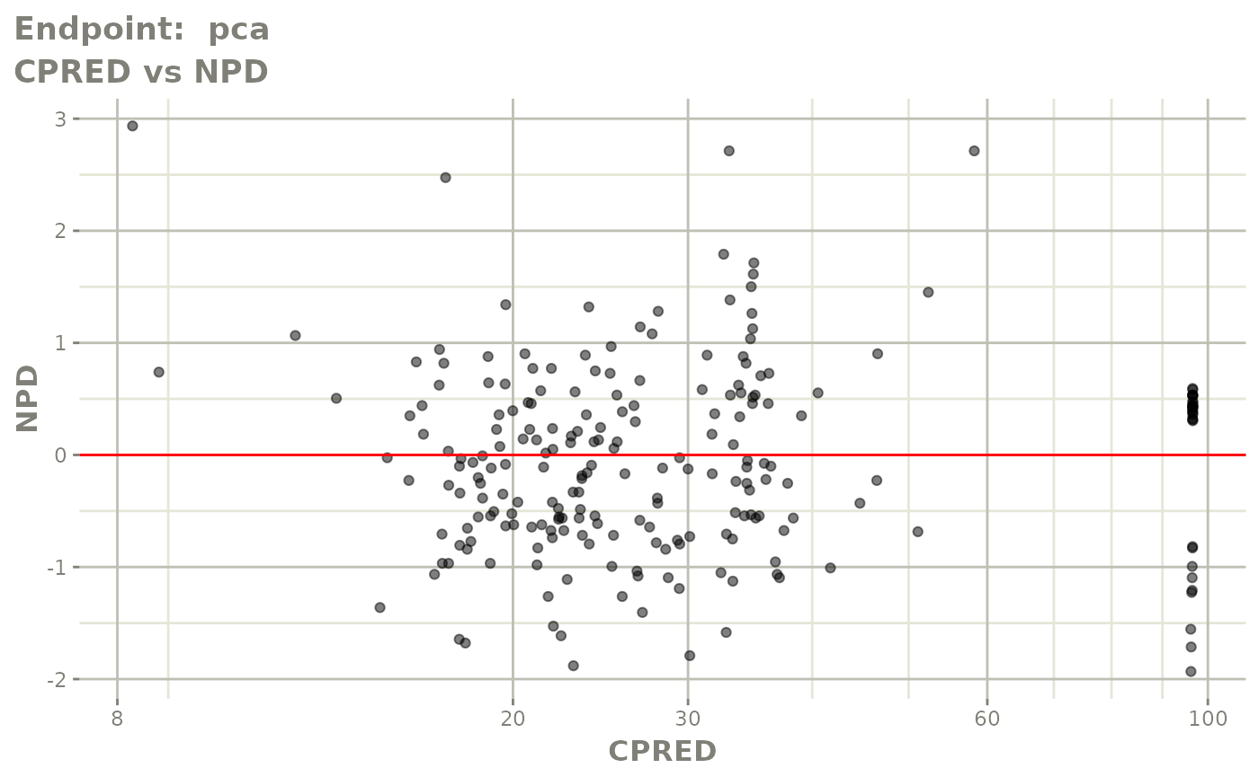
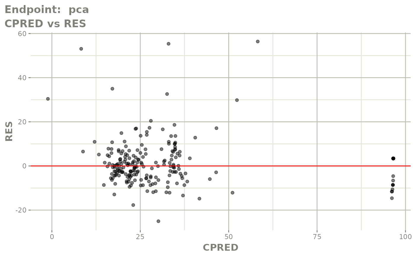
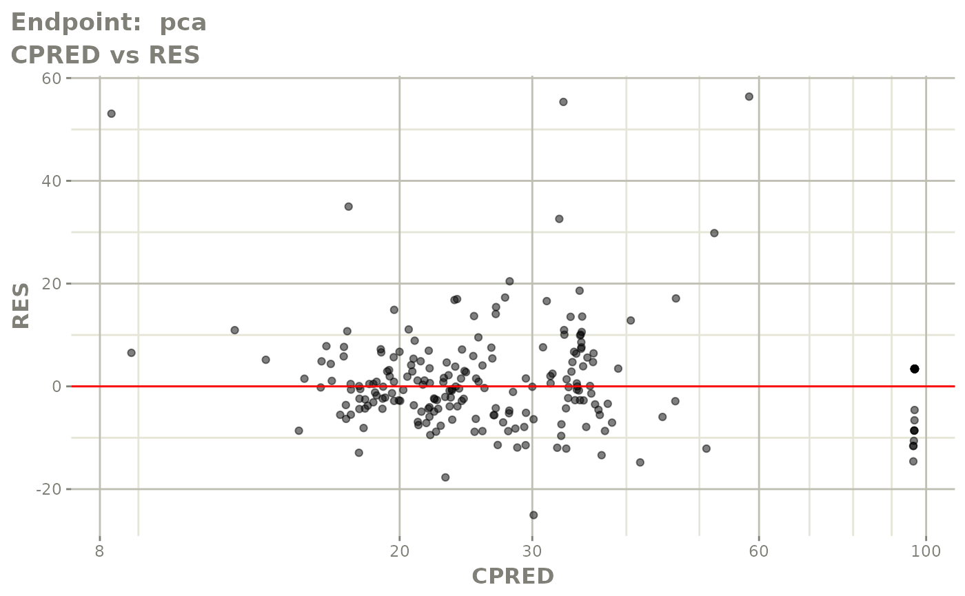
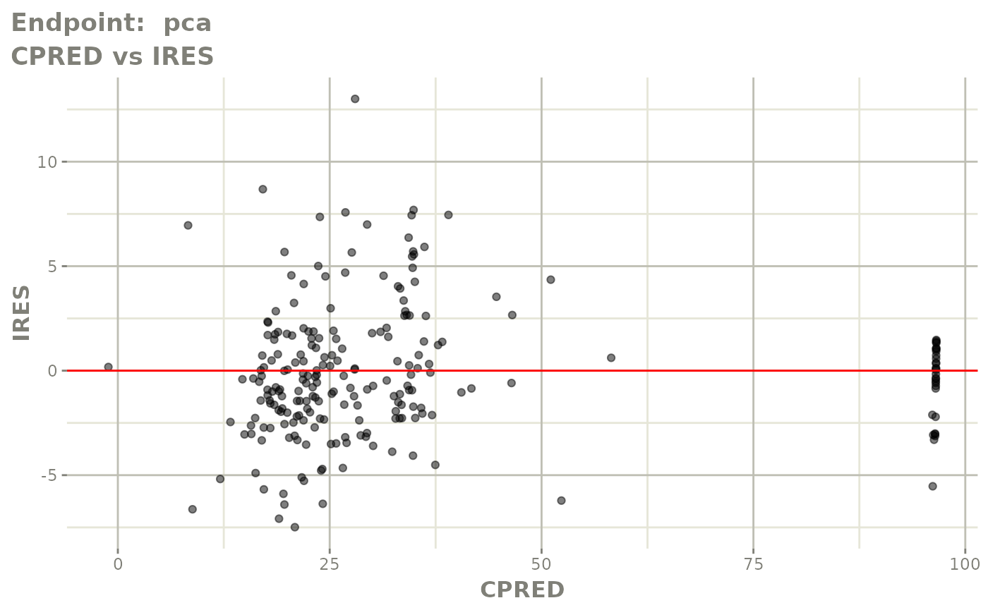
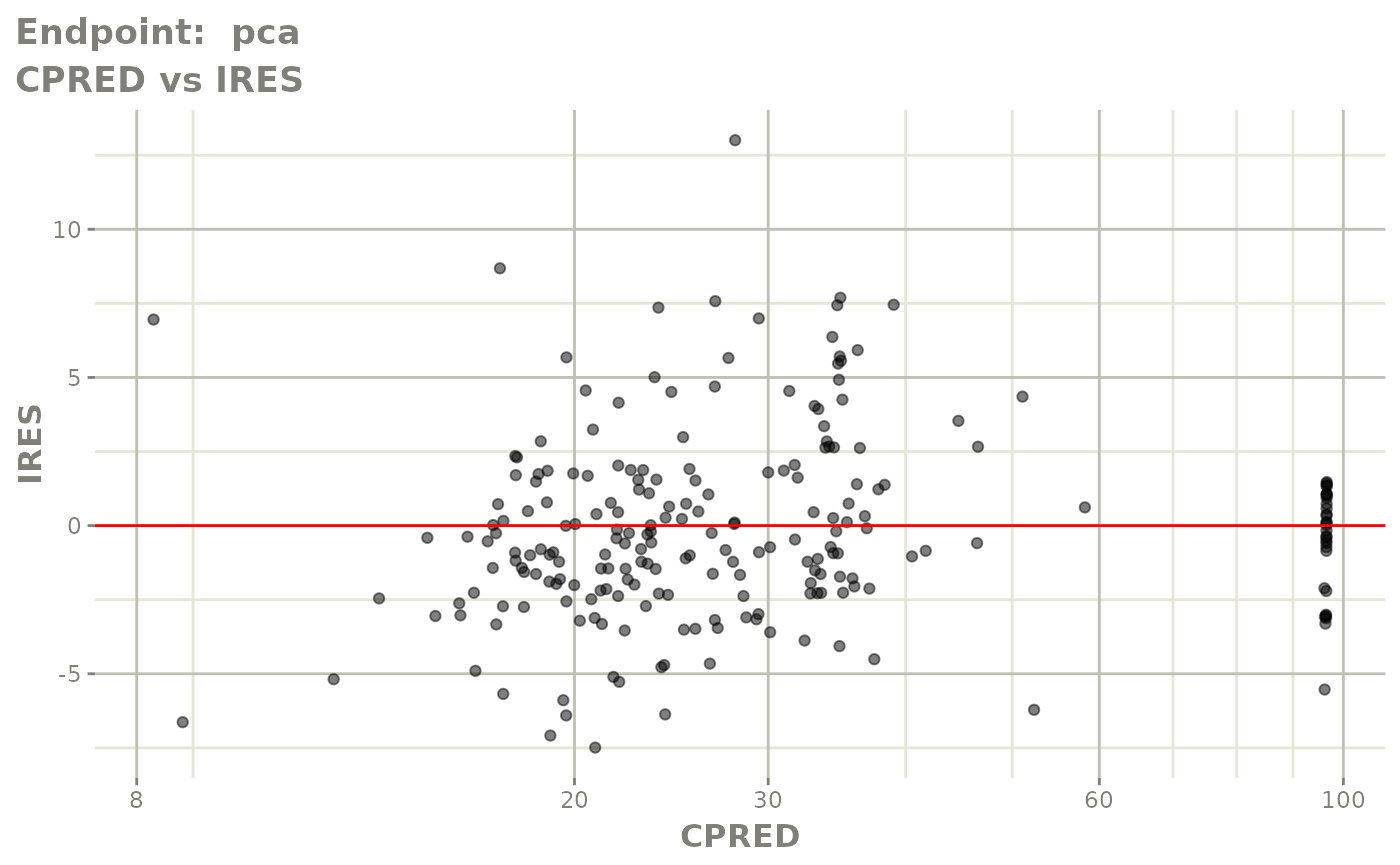
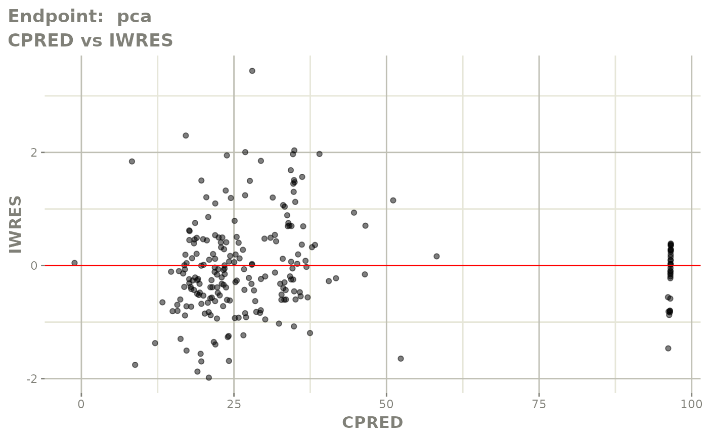
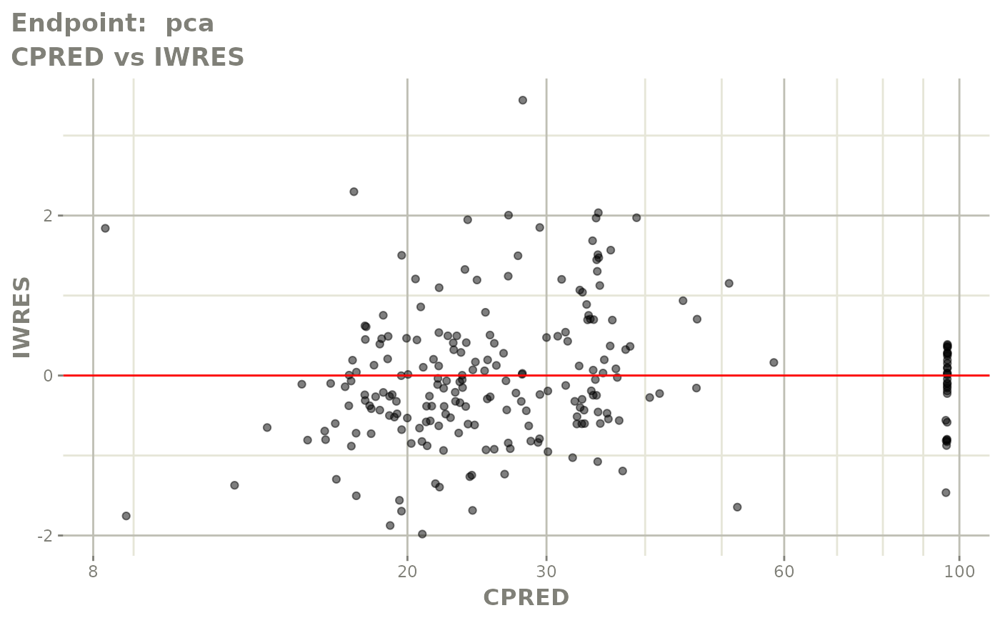
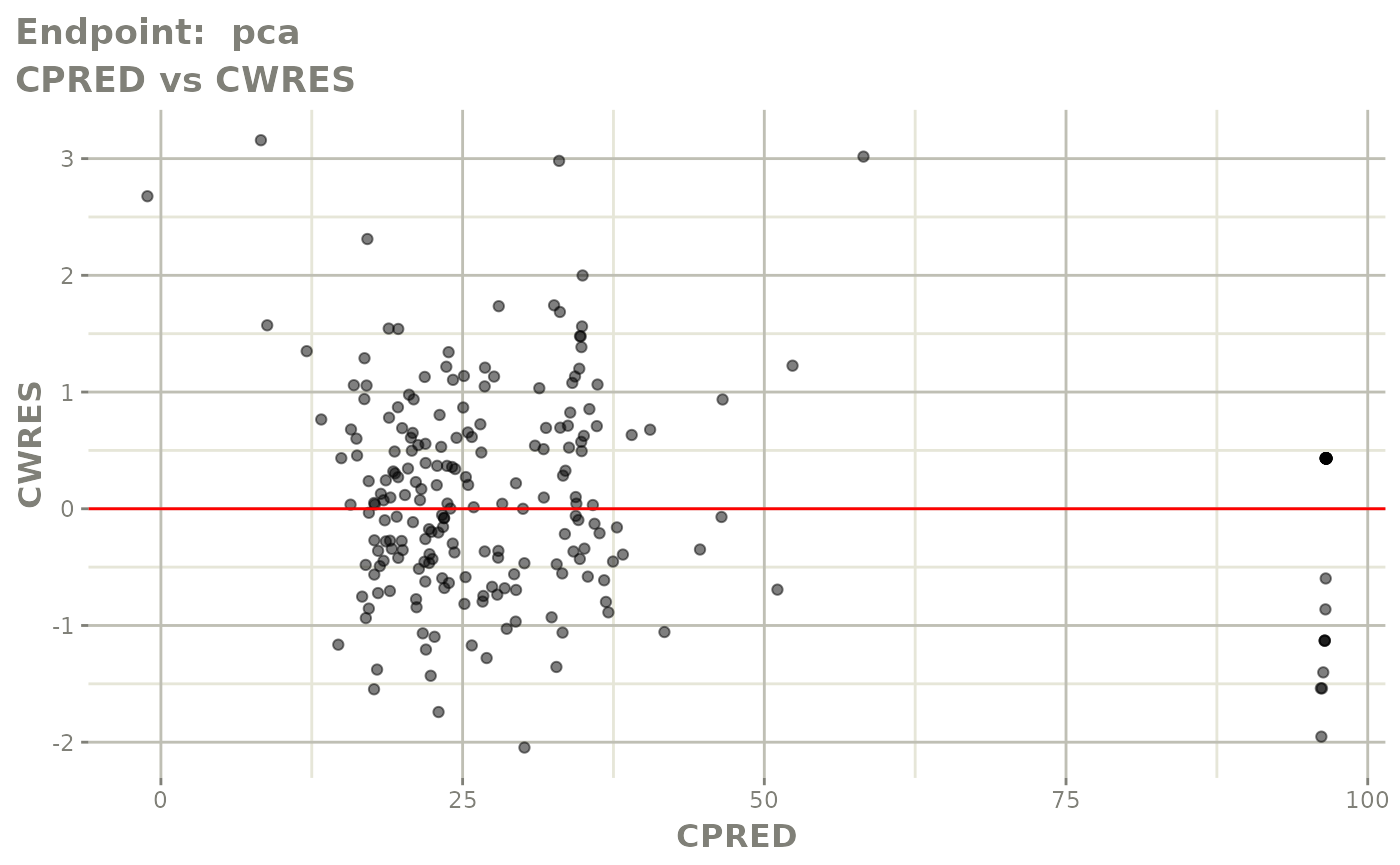
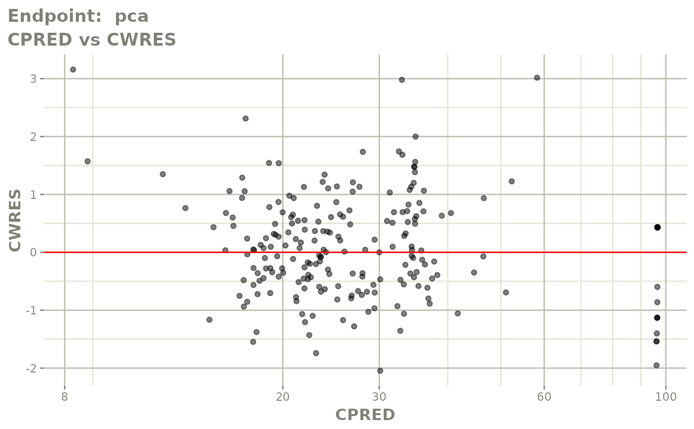
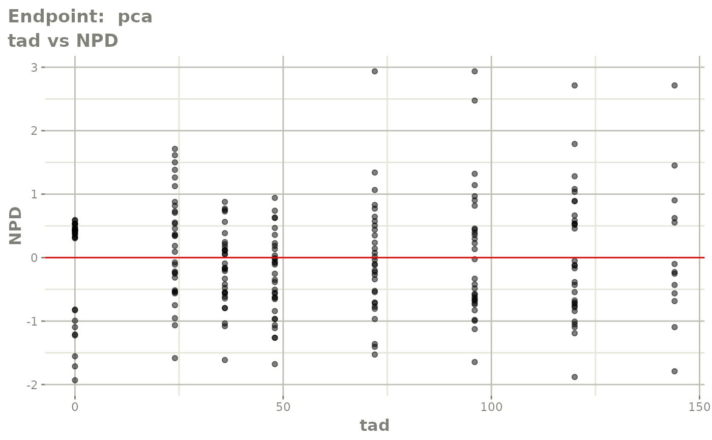
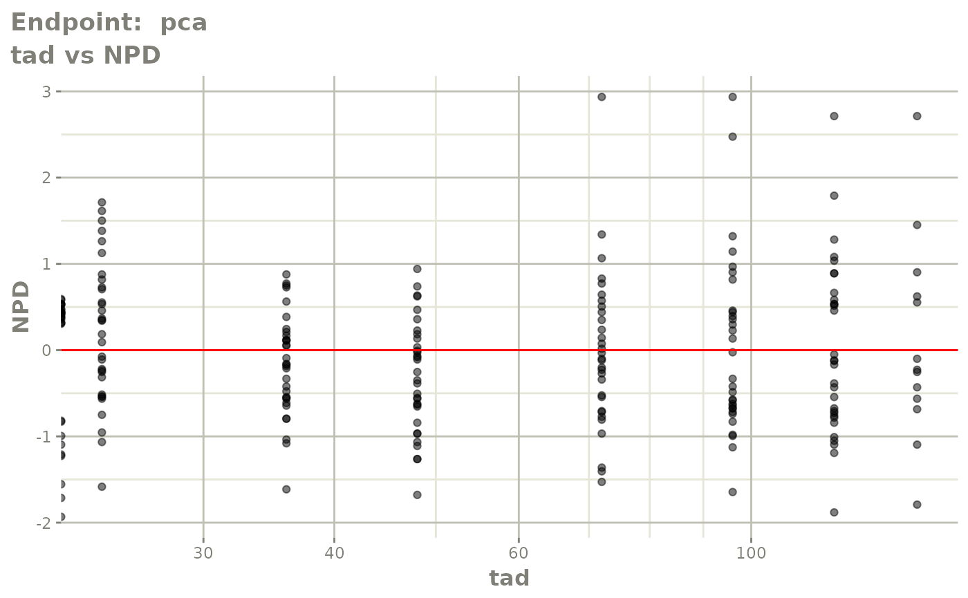
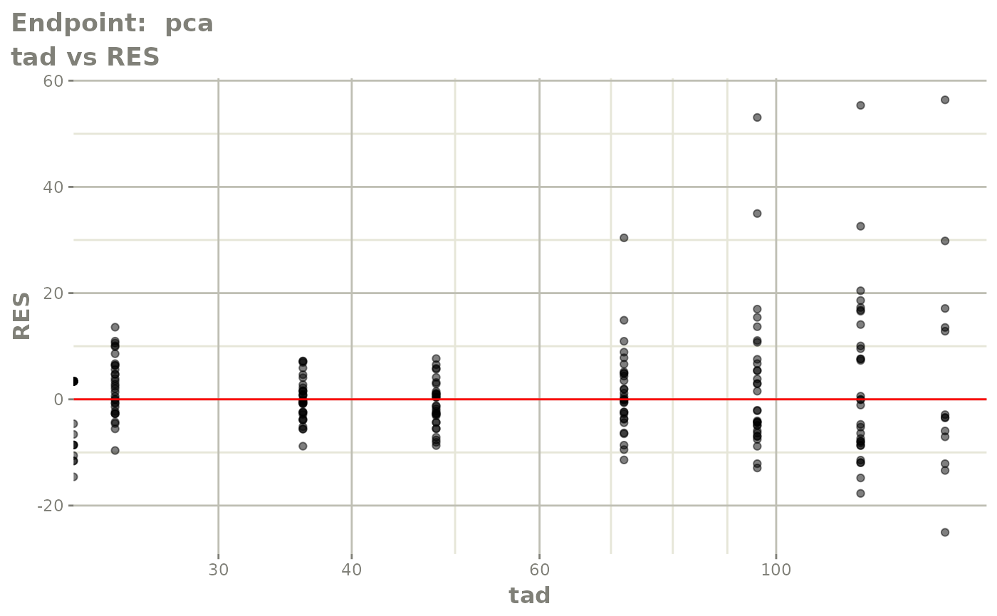
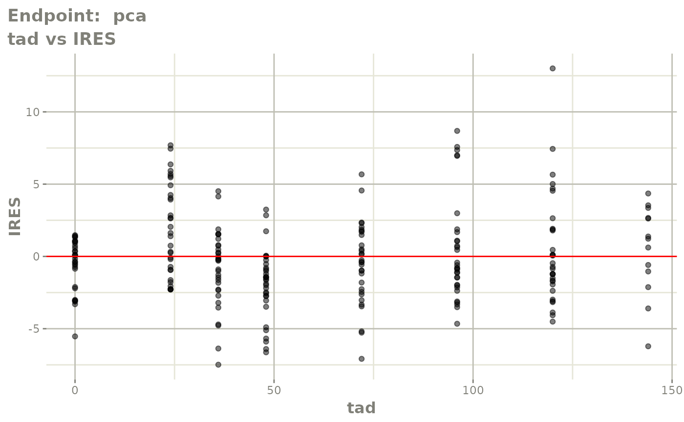
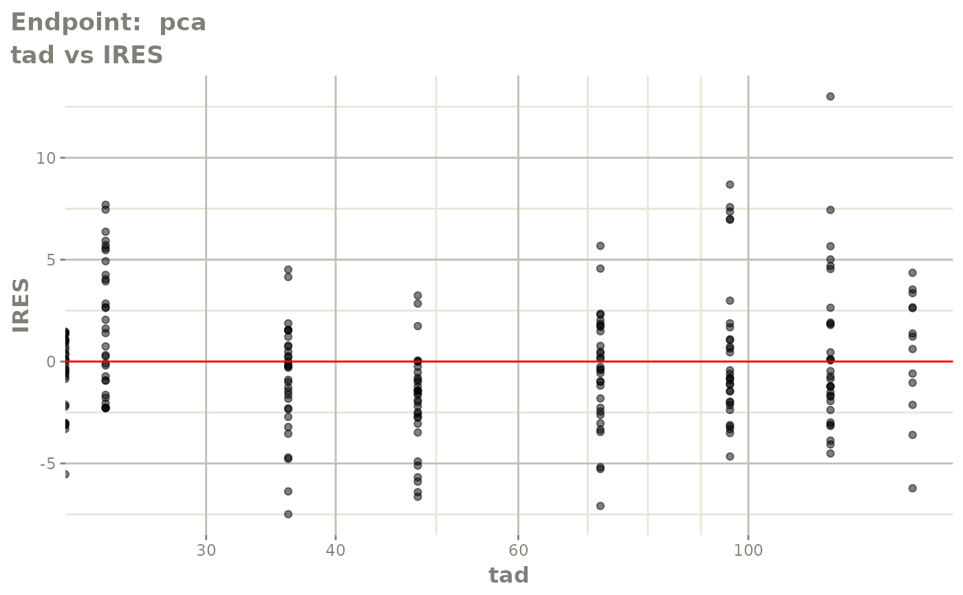
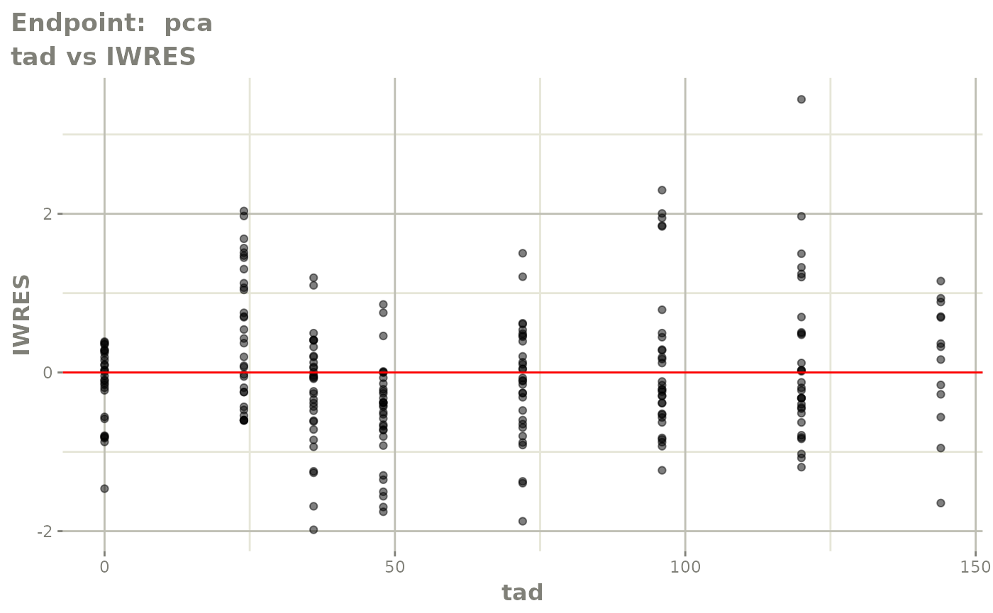
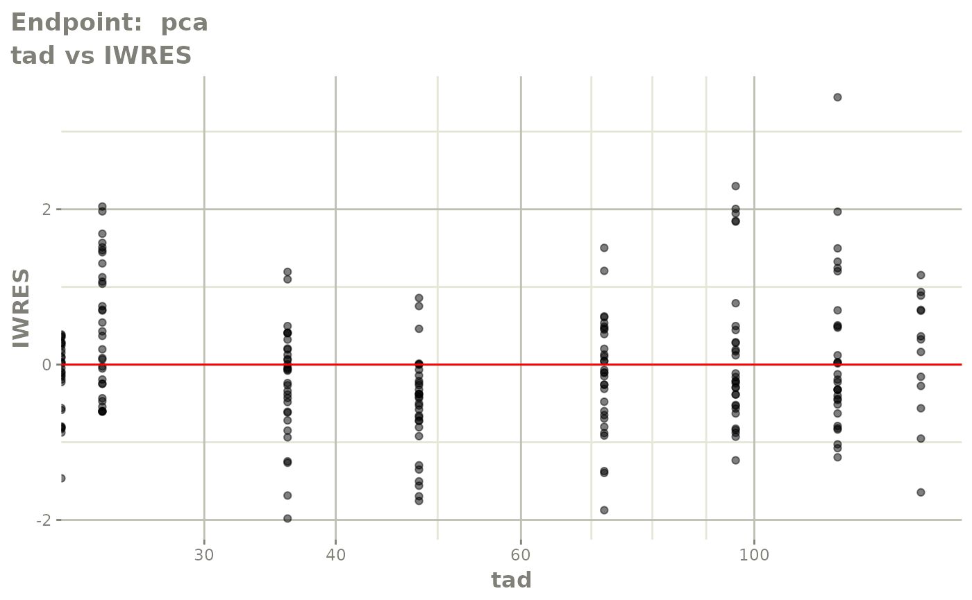
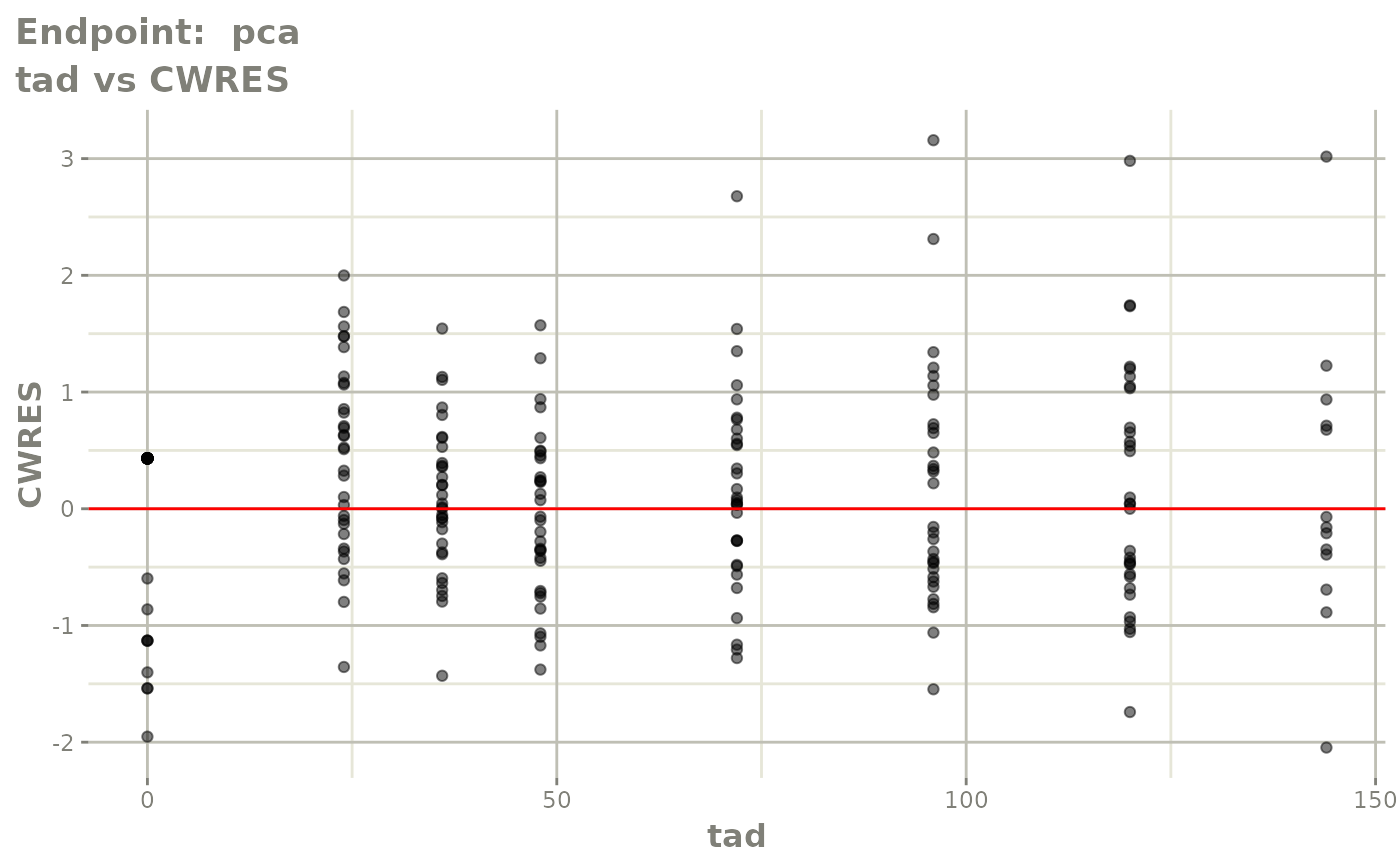
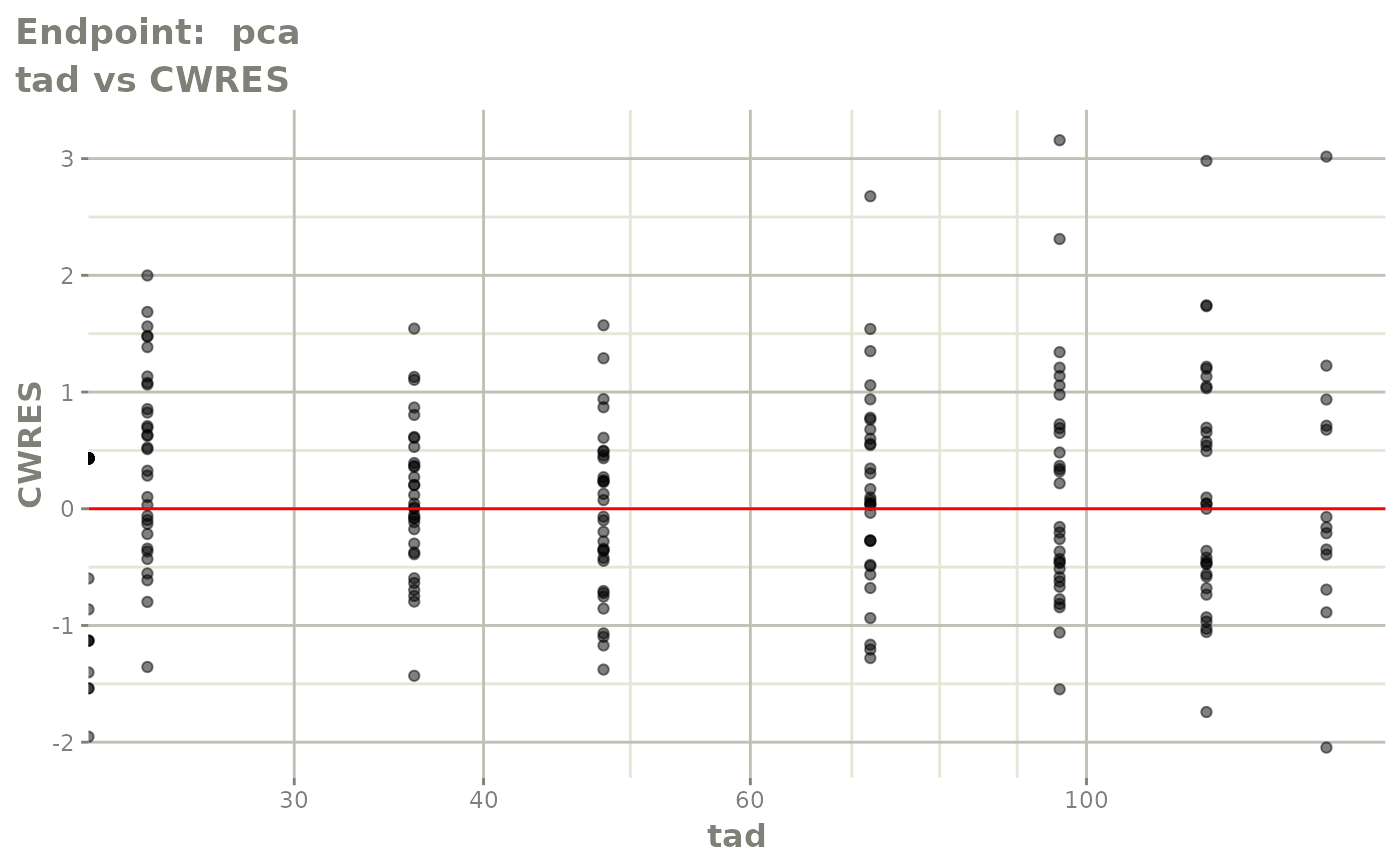
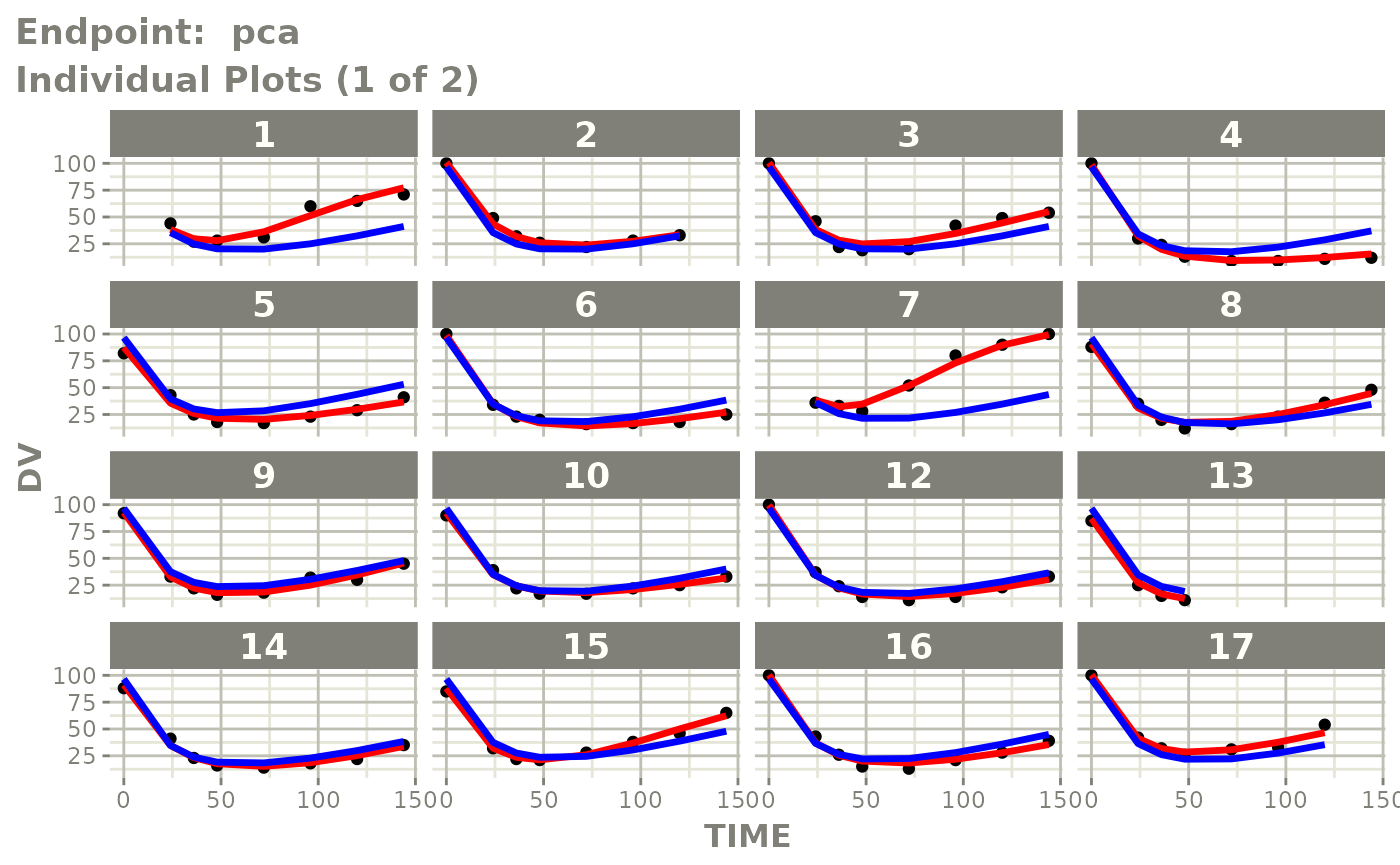
#> # e0 <dbl>, DCP <dbl>, PD.1 <dbl>, kin <dbl>, tad <dbl>, dosenum <dbl>SAEM Diagnostic plots
plot(fit.TOS)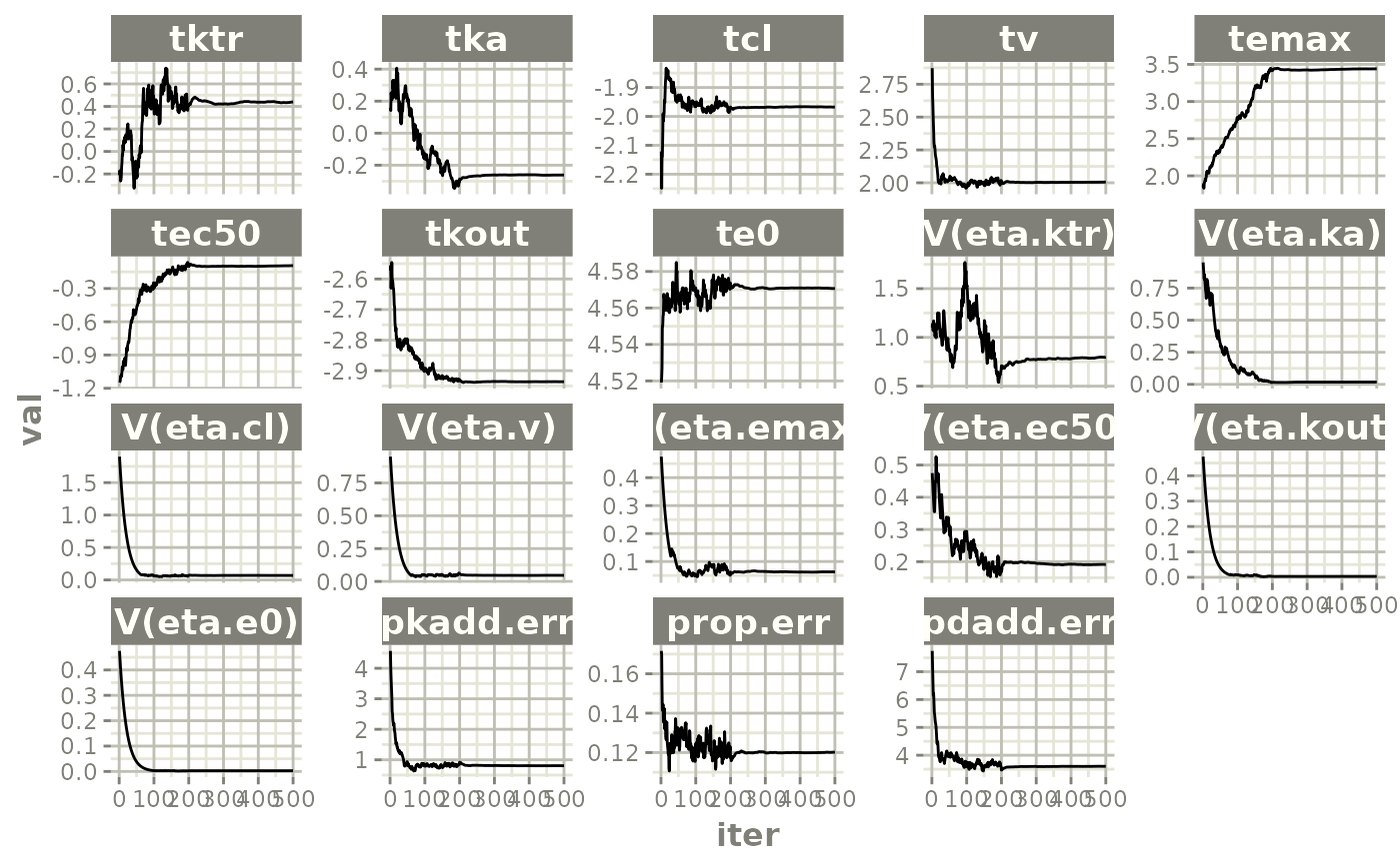


v1s <- vpcPlot(fit.TOS, show=list(obs_dv=TRUE), scales="free_y") +
ylab("Warfarin Cp [mg/L] or PCA") +
xlab("Time [h]")
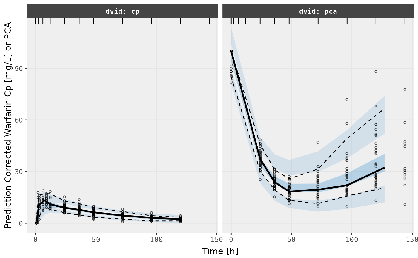
v2s <- vpcPlot(fit.TOS, show=list(obs_dv=TRUE), pred_corr = TRUE) +
ylab("Prediction Corrected Warfarin Cp [mg/L] or PCA") +
xlab("Time [h]")
v1s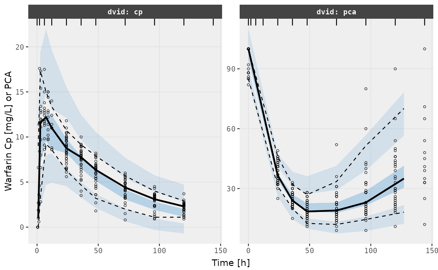
v2s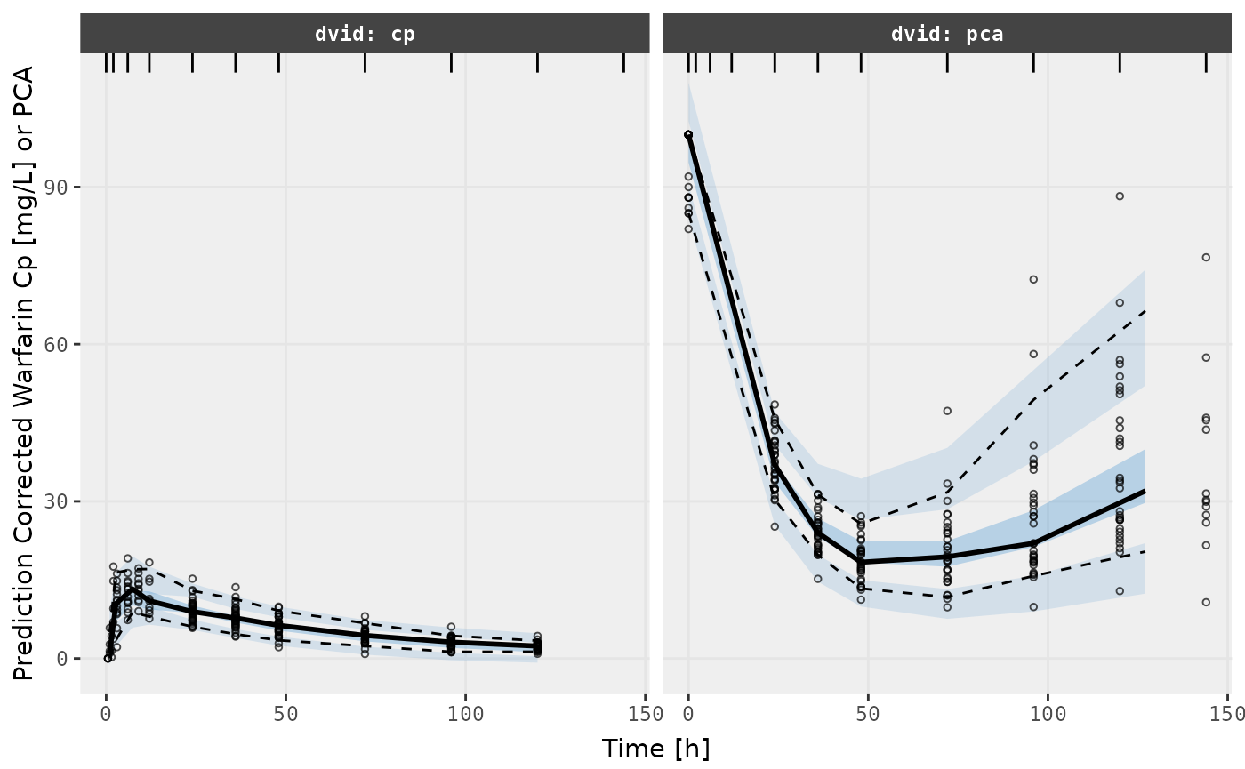
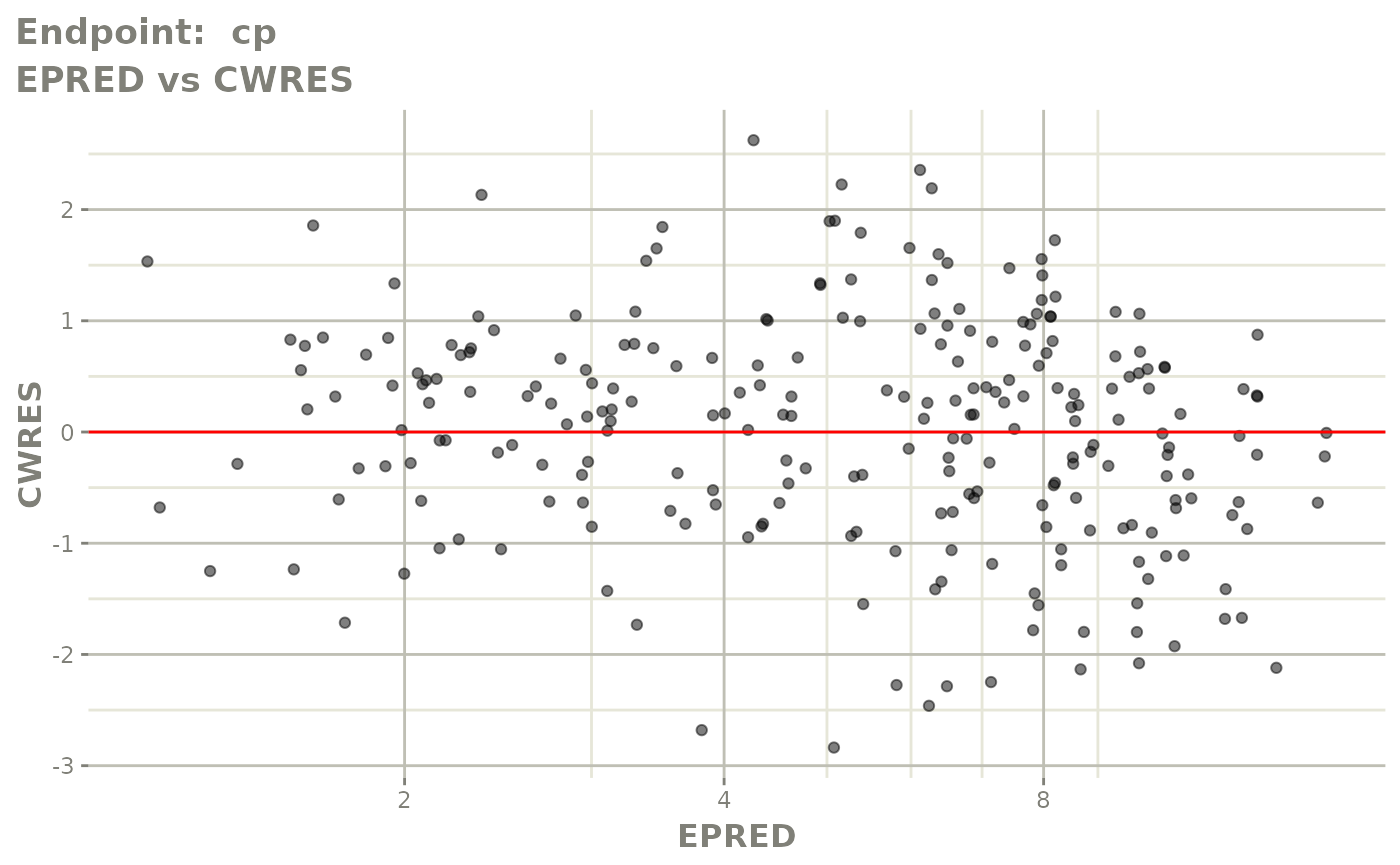
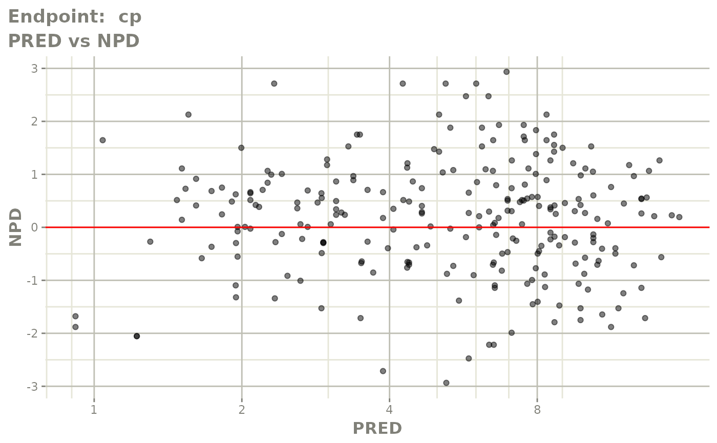
FOCEi fits
## FOCEi fit/vpcs
fit.TOF <- nlmixr(pk.turnover.emax3, warfarin, "focei", control=list(print=0),
table=list(cwres=TRUE, npde=TRUE))
#> calculating covariance matrix
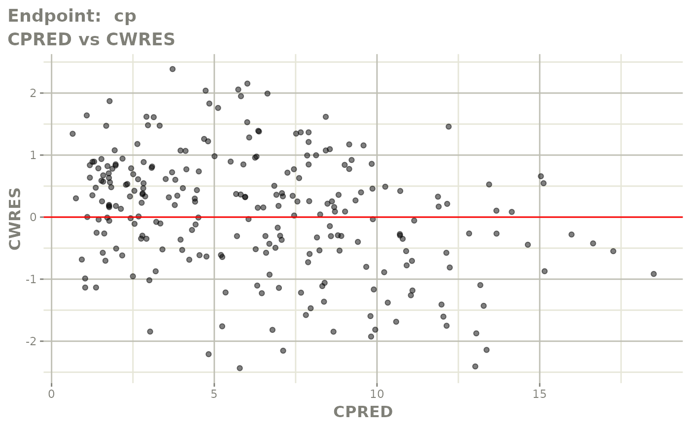
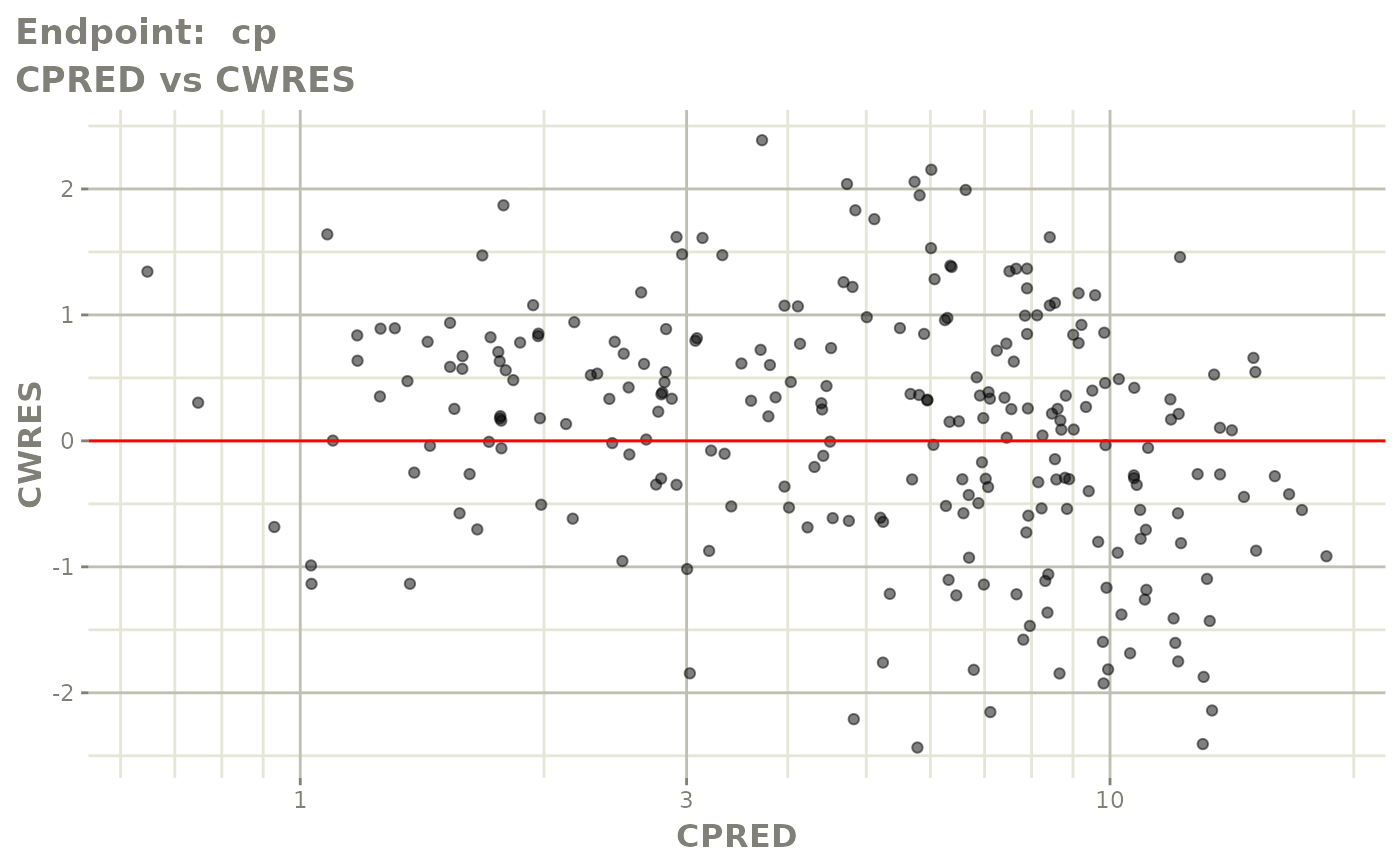
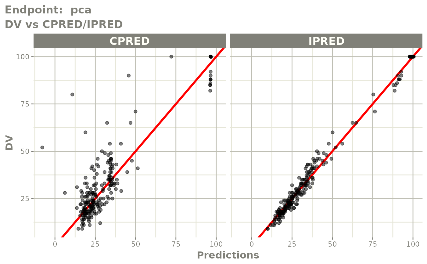
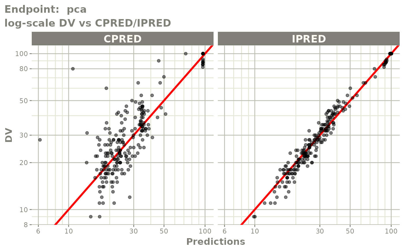
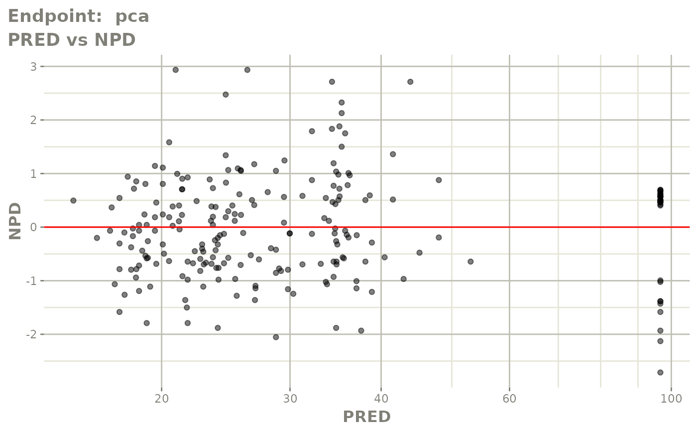
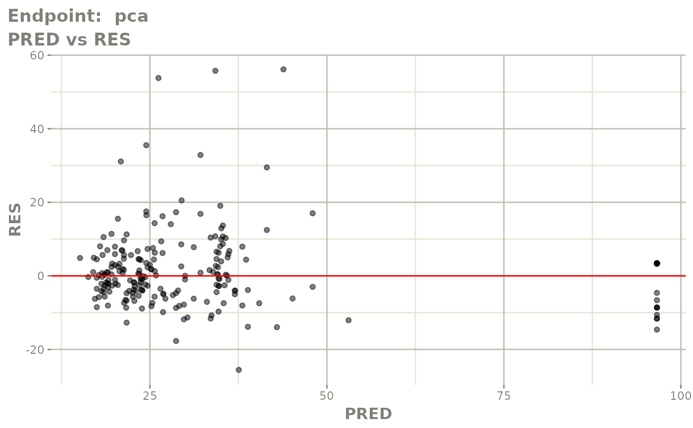
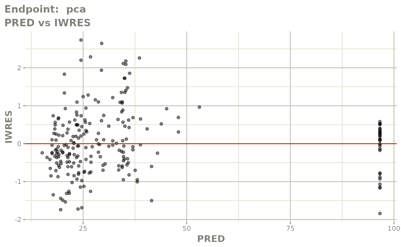
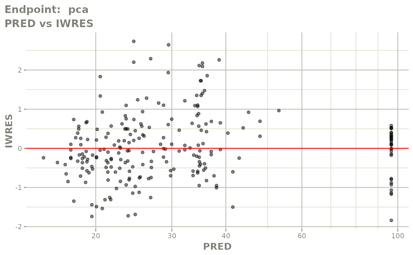
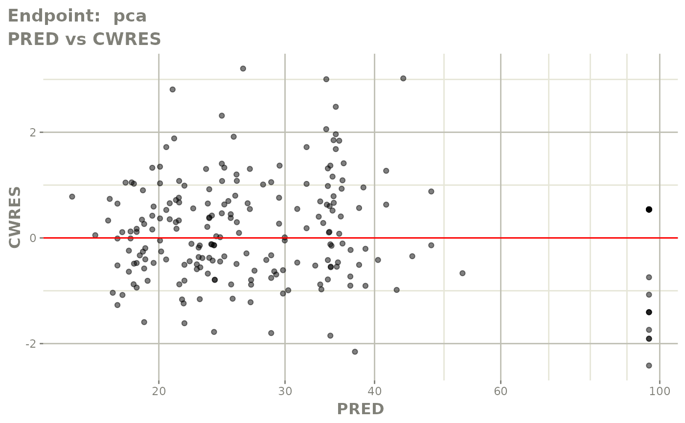
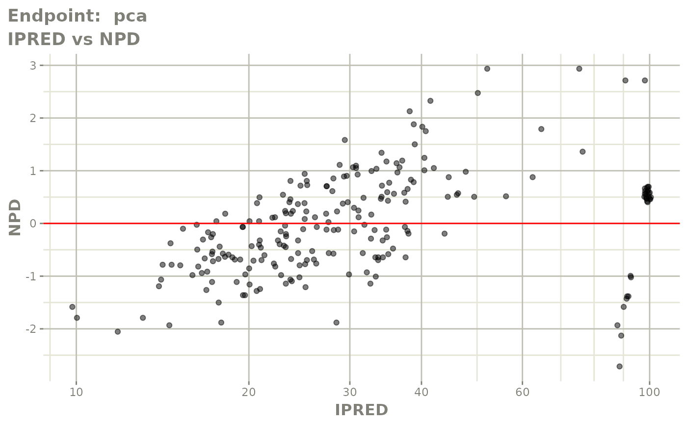
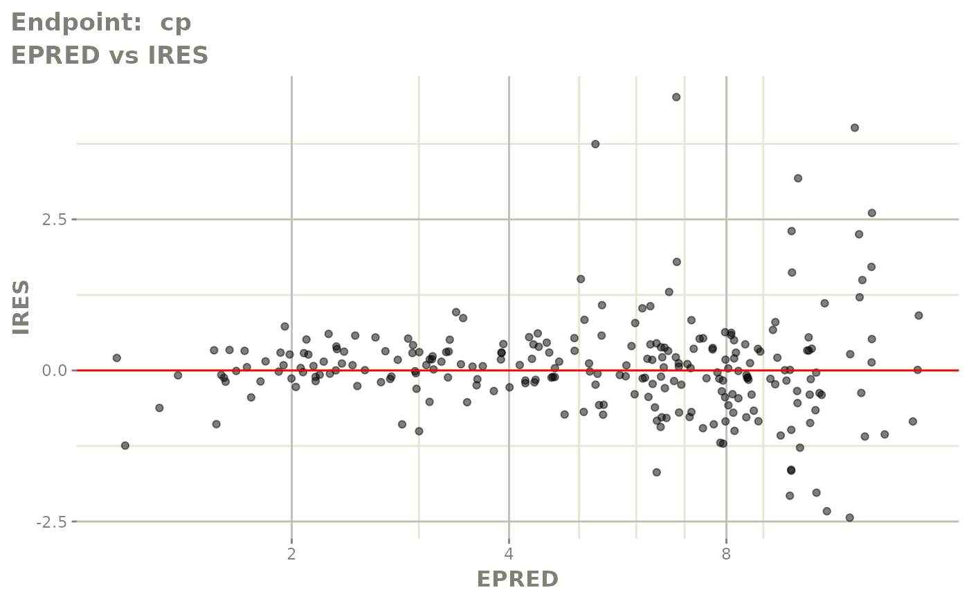
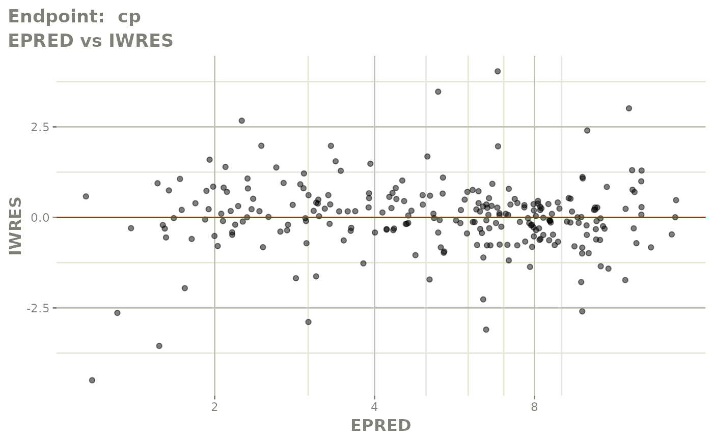
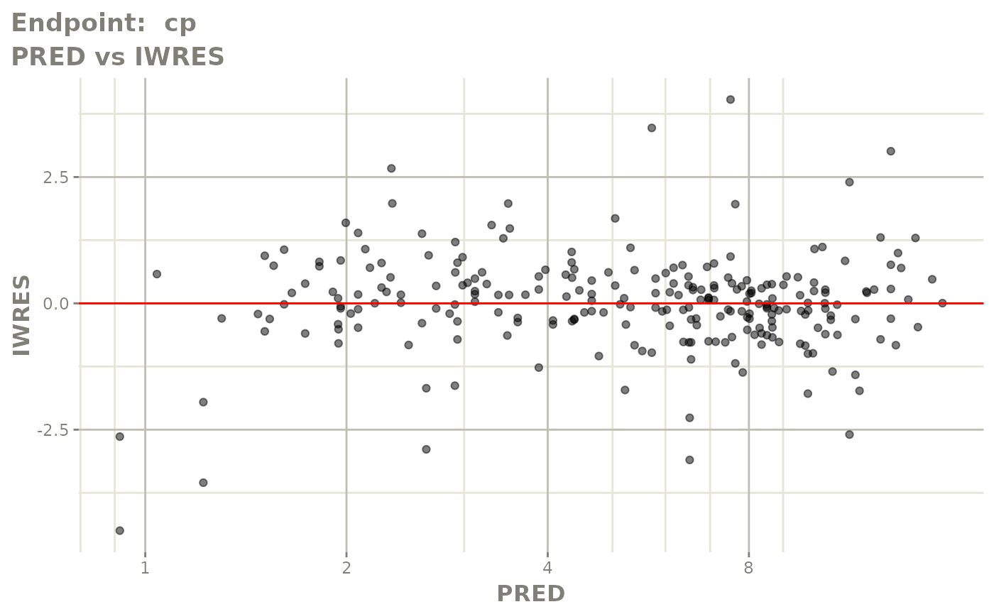
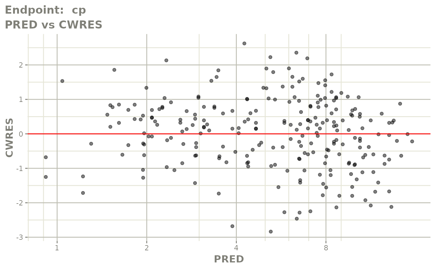
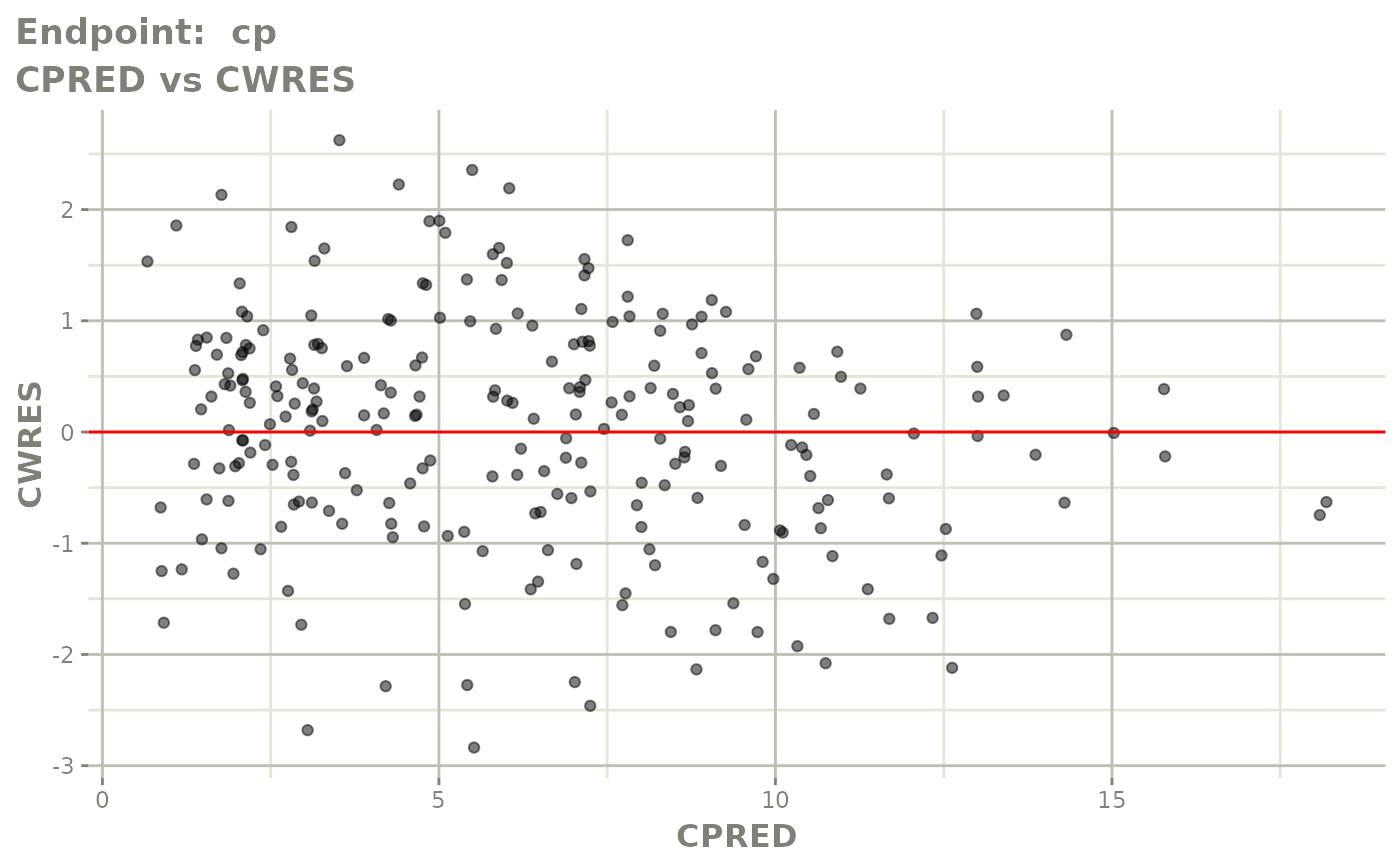
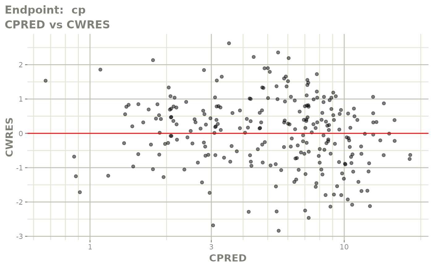
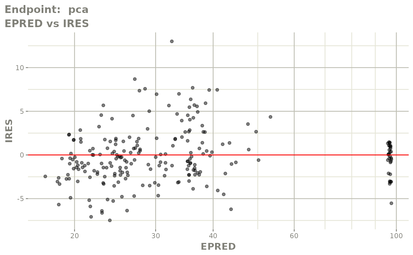
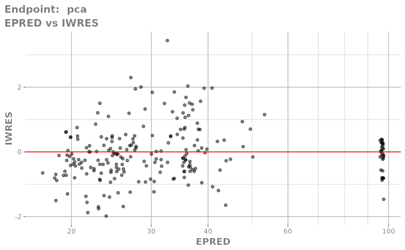
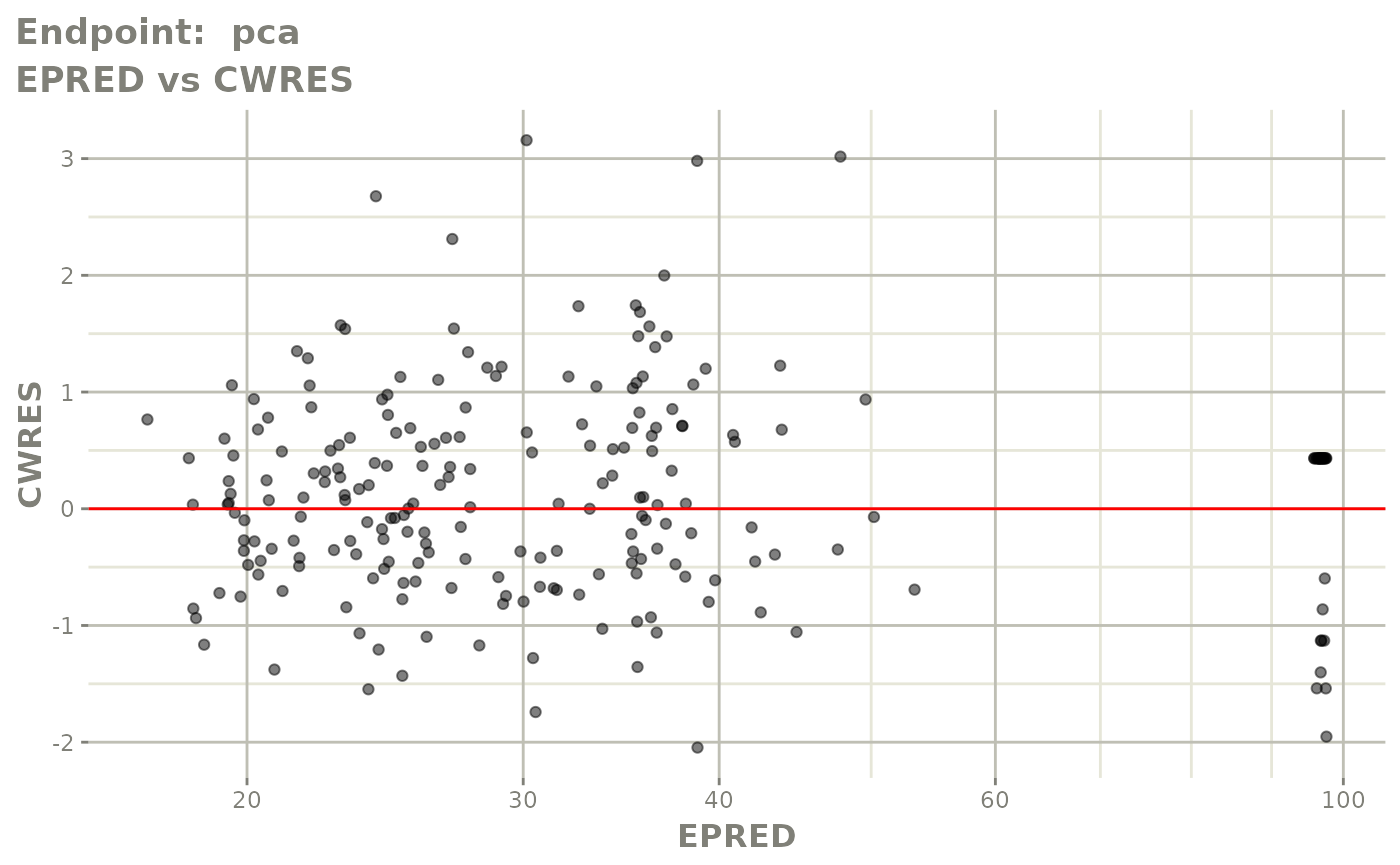
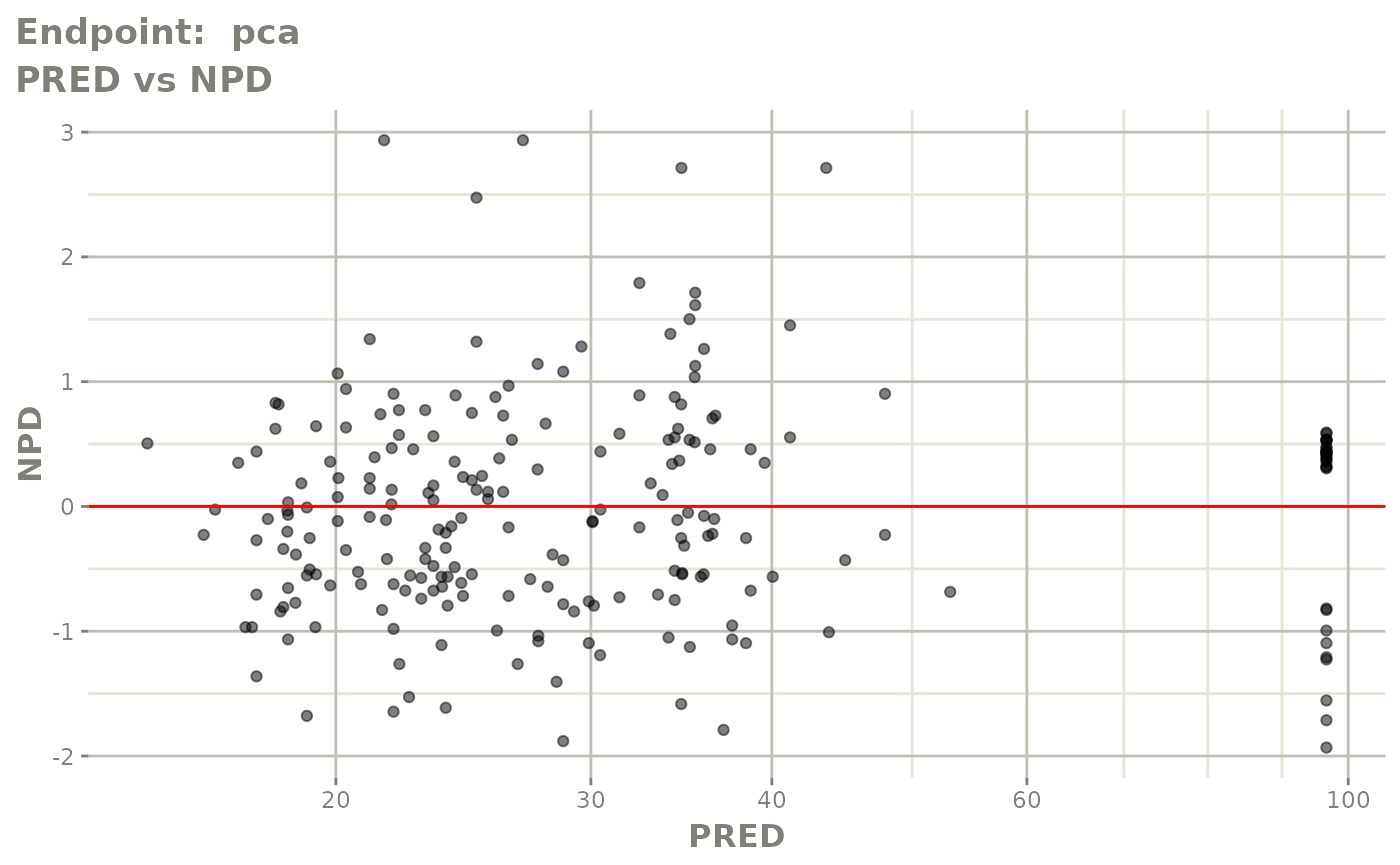
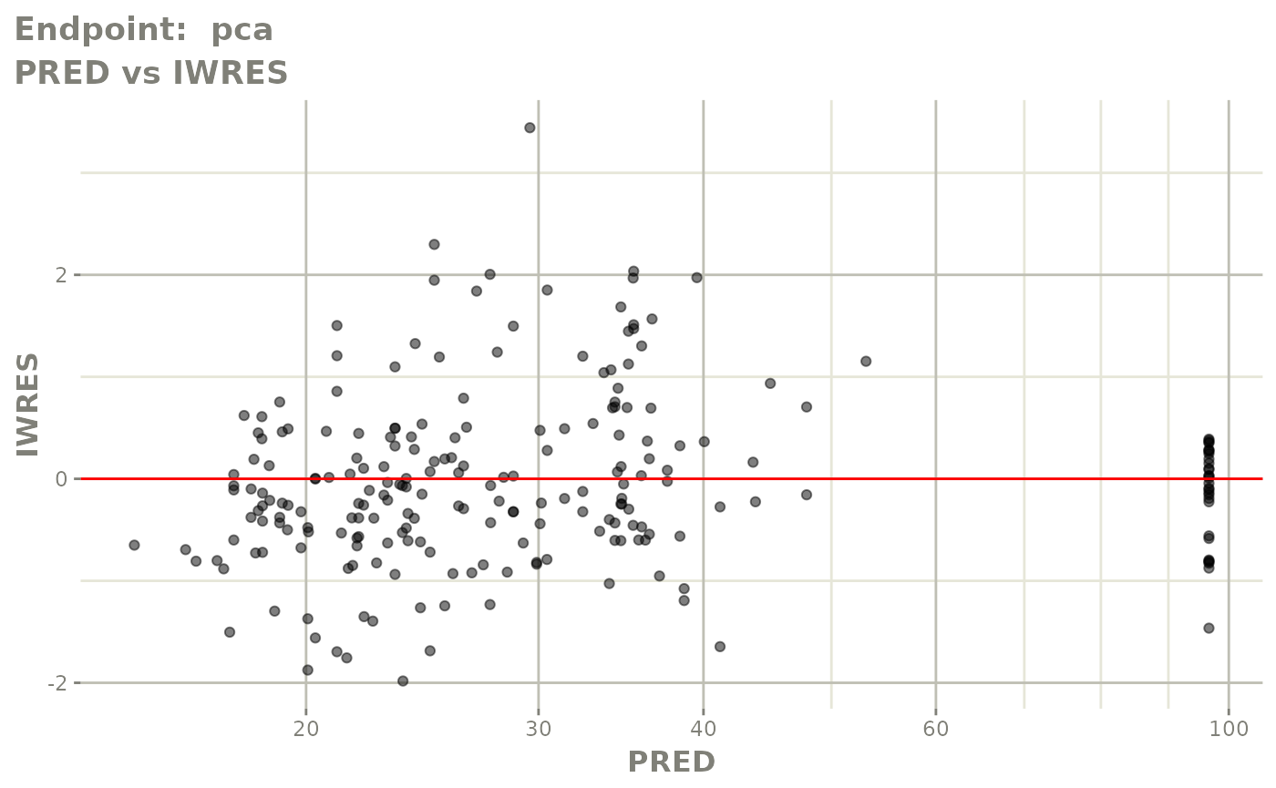
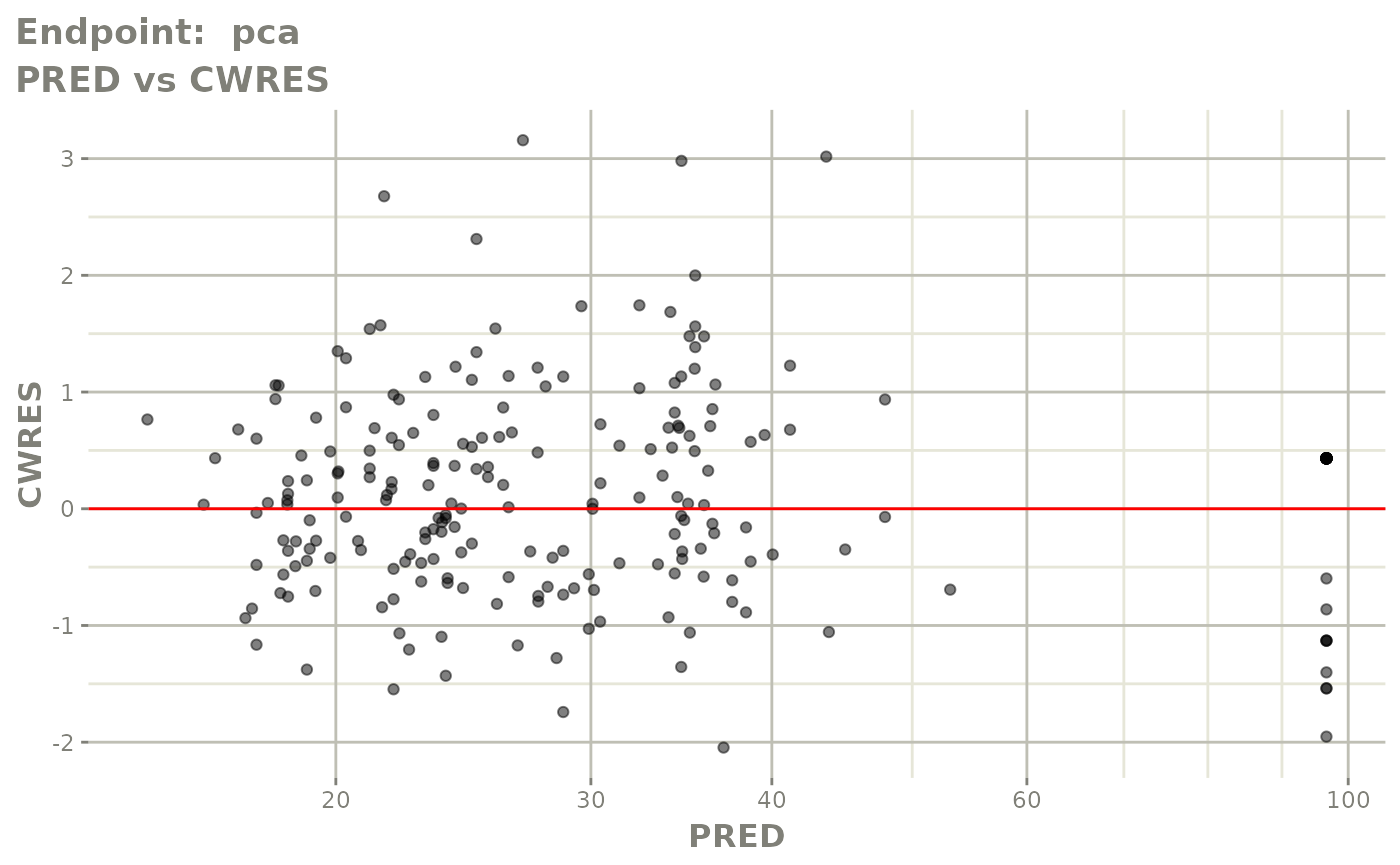
#> doneFOCEi Diagnostic Plots
print(fit.TOF)
#> ── nlmixr² FOCEi (outer: nlminb) ──
#>
#> OBJF AIC BIC Log-likelihood Condition#(Cov) Condition#(Cor)
#> FOCEi 1374.783 2300.478 2379.898 -1131.239 100298.2 872.8198
#>
#> ── Time (sec $time): ──
#>
#> setup optimize covariance table compress other
#> elapsed 0.002758 55.83564 55.83564 1.494 0.011 317.871
#>
#> ── Population Parameters ($parFixed or $parFixedDf): ──
#>
#> Est. SE %RSE Back-transformed(95%CI) BSV(CV% or SD)
#> tktr 0.168 0.136 80.9 1.18 (0.906, 1.54) 107.
#> tka -0.0713 0.149 209 0.931 (0.695, 1.25) 91.5
#> tcl -2.01 0.0328 1.63 0.134 (0.125, 0.142) 26.9
#> tv 2.07 0.0234 1.13 7.96 (7.61, 8.34) 22.2
#> prop.err 0.135 0.135
#> pkadd.err 0.22 0.22
#> temax 5.42 0.587 10.8 0.996 (0.986, 0.999) 0.644
#> tec50 0.144 0.0541 37.5 1.16 (1.04, 1.28) 45.5
#> tkout -2.94 0.0285 0.97 0.0529 (0.0501, 0.056) 10.6
#> te0 4.57 0.0166 0.363 96.6 (93.5, 99.8) 7.08
#> pdadd.err 3.78 3.78
#> Shrink(SD)%
#> tktr 60.3%
#> tka 61.3%
#> tcl -2.84%
#> tv 6.29%
#> prop.err
#> pkadd.err
#> temax 96.9%
#> tec50 3.27%
#> tkout 28.8%
#> te0 25.5%
#> pdadd.err
#>
#> Covariance Type ($covMethod): r,s
#> No correlations in between subject variability (BSV) matrix
#> Full BSV covariance ($omega) or correlation ($omegaR; diagonals=SDs)
#> Distribution stats (mean/skewness/kurtosis/p-value) available in $shrink
#> Information about run found ($runInfo):
#> • gradient problems with initial estimate and covariance; see $scaleInfo
#> • last objective function was not at minimum, possible problems in optimization
#> • ETAs were reset to zero during optimization; (Can control by foceiControl(resetEtaP=.))
#> • initial ETAs were nudged; (can control by foceiControl(etaNudge=., etaNudge2=))
#> Censoring ($censInformation): No censoring
#> Minimization message ($message):
#> false convergence (8)
#> In an ODE system, false convergence may mean "useless" evaluations were performed.
#> See https://tinyurl.com/yyrrwkce
#> It could also mean the convergence is poor, check results before accepting fit
#> You may also try a good derivative free optimization:
#> nlmixr2(...,control=list(outerOpt="bobyqa"))
#>
#> ── Fit Data (object is a modified tibble): ──
#> # A tibble: 483 × 44
#> ID TIME CMT DV EPRED ERES NPDE NPD PDE PD PRED RES
#> <fct> <dbl> <fct> <dbl> <dbl> <dbl> <dbl> <dbl> <dbl> <dbl> <dbl> <dbl>
#> 1 1 0.5 cp 0 1.76 -1.76 -1.64 -2.05 0.05 0.02 1.22 -1.22
#> 2 1 1 cp 1.9 3.93 -2.03 1.99 -0.643 0.977 0.26 3.51 -1.61
#> 3 1 2 cp 3.3 7.16 -3.86 -2.33 -1.07 0.01 0.143 7.63 -4.33
#> # ℹ 480 more rows
#> # ℹ 32 more variables: WRES <dbl>, IPRED <dbl>, IRES <dbl>, IWRES <dbl>,
#> # CPRED <dbl>, CRES <dbl>, CWRES <dbl>, eta.ktr <dbl>, eta.ka <dbl>,
#> # eta.cl <dbl>, eta.v <dbl>, eta.emax <dbl>, eta.ec50 <dbl>, eta.kout <dbl>,
#> # eta.e0 <dbl>, depot <dbl>, gut <dbl>, center <dbl>, effect <dbl>,
#> # ktr <dbl>, ka <dbl>, cl <dbl>, v <dbl>, emax <dbl>, ec50 <dbl>, kout <dbl>,
#> # e0 <dbl>, DCP <dbl>, PD.1 <dbl>, kin <dbl>, tad <dbl>, dosenum <dbl>
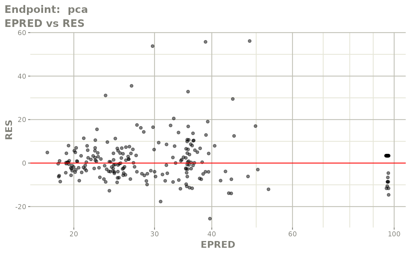
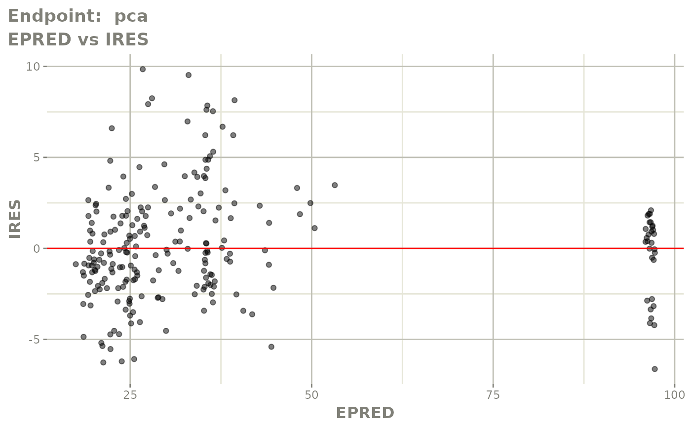
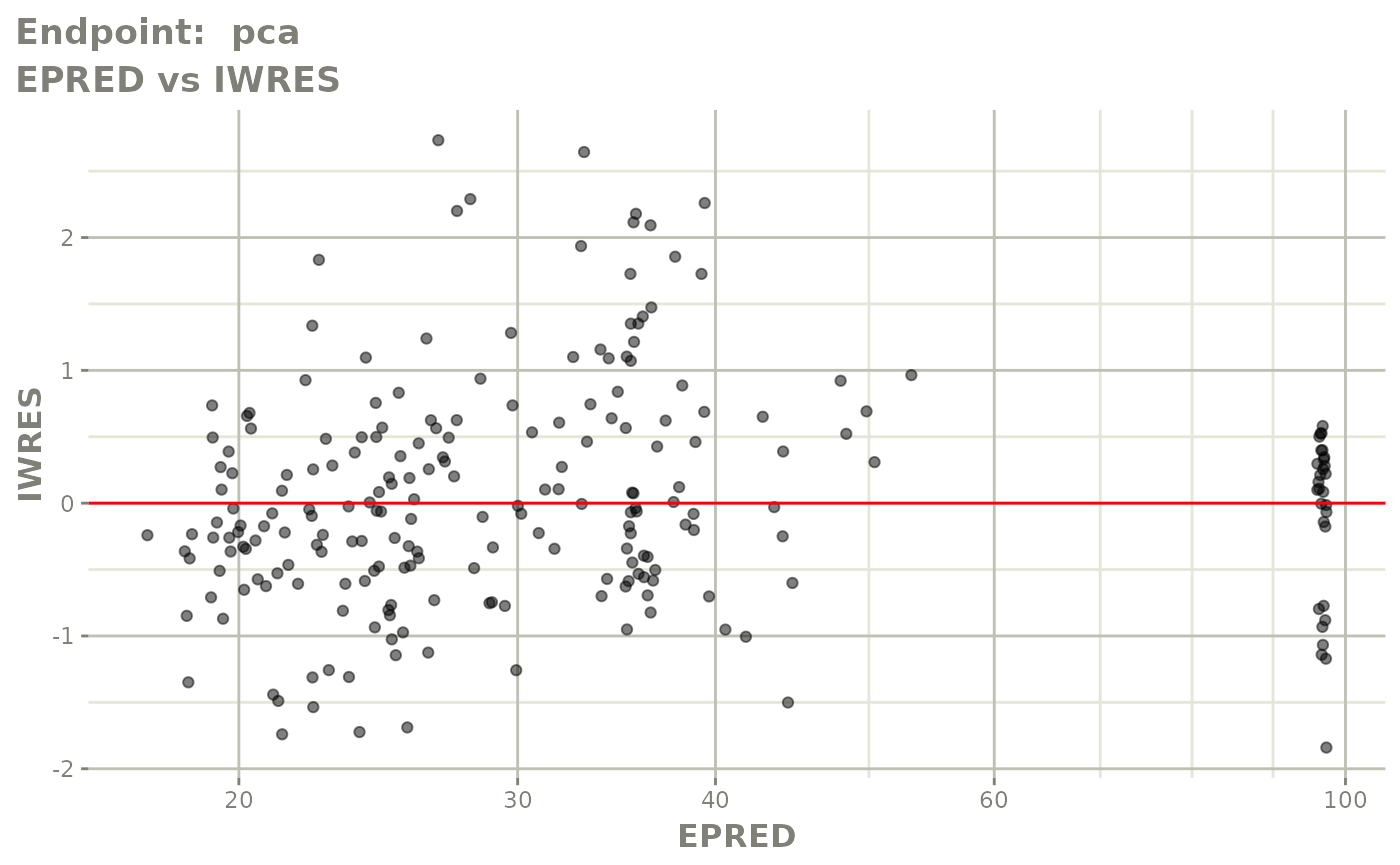
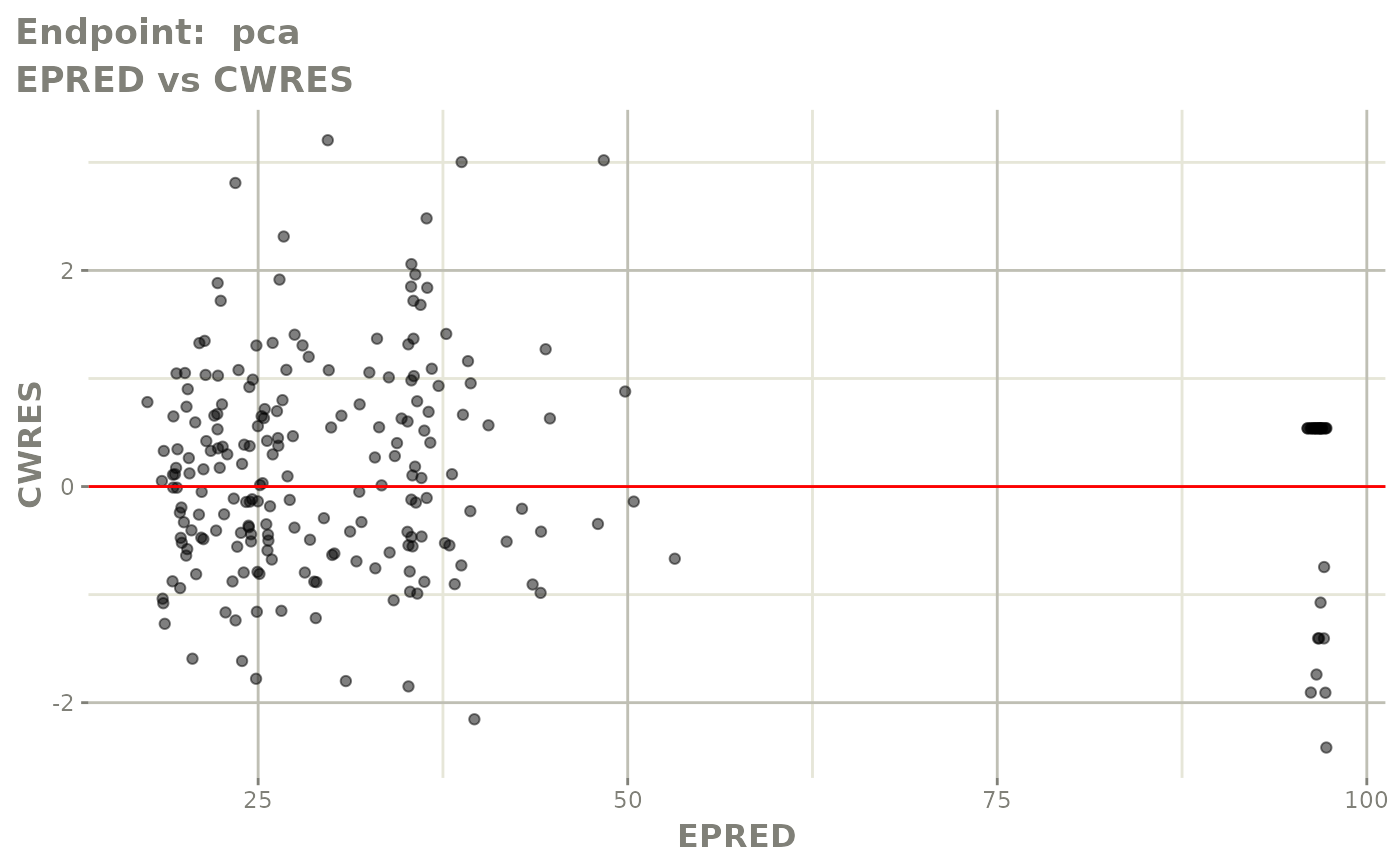
plot(fit.TOF)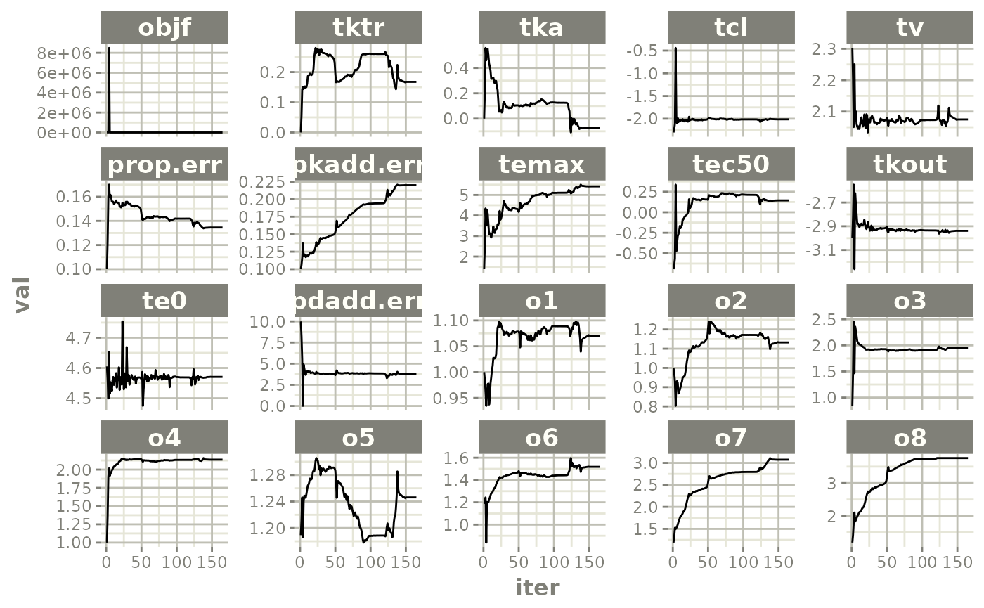


v1f <- vpcPlot(fit.TOF, show=list(obs_dv=TRUE), scales="free_y") +
  ylab("Warfarin Cp [mg/L] or PCA") +
  xlab("Time [h]")

v2f <- vpcPlot(fit.TOF, show=list(obs_dv=TRUE), pred_corr = TRUE) +
  ylab("Prediction Corrected Warfarin Cp [mg/L] or PCA") +
  xlab("Time [h]")

v1f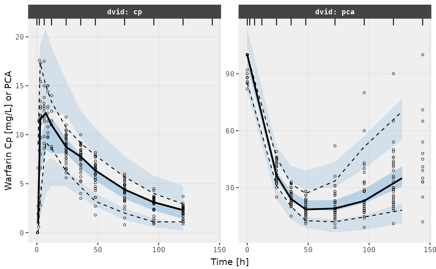
v2f