This vignette is meant to be the smallest useful package-side
introduction to np. The emphasis is on one clean workflow
that users can run after installation: choose a bandwidth, fit a model,
inspect the result, and plot it.
Broader worked examples, package comparisons, and method-specific articles are better carried by the gallery site:
- https://jeffreyracine.github.io/gallery/np_npRmpi.html
- https://jeffreyracine.github.io/gallery/quickstarts.html
The basic workflow
In np, the bandwidth object is often the key object in
the analysis.
- compute or inspect a bandwidth object,
- fit the model,
- summarize or plot the result.
A simple regression example
library(np)
#> np 0.70-4
#> Examples and guides at https://jeffreyracine.github.io/gallery/
#> See also vignette("np_getting_started", package = "np")
data(cps71, package = "np")

bw <- npregbw(logwage ~ age, data = cps71)
summary(bw)
#>
#> Regression Data (205 observations, 1 variable(s)):
#>
#> Regression Type: Local-Constant
#> Bandwidth Selection Method: Least Squares Cross-Validation
#> Formula: logwage ~ age
#> Bandwidth Type: Fixed
#> Objective Function Value: 0.316055 (achieved on multistart 1)
#> Number of Function Evaluations: 47
#> Powell cache: 17 repeated objective lookups avoided out of 41 (41.5%)
#>
#> Exp. Var. Name: age Bandwidth: 1.892158  Scale Factor: 0.4487743
#>
#> Continuous Kernel Type: Second-Order Gaussian
#> No. Continuous Explanatory Vars.: 1
#> Estimation Time: 0.268 seconds

fit <- npreg(bws = bw)
summary(fit)
#>
#> Regression Data: 205 training points, in 1 variable(s)
#>                    age
#> Bandwidth(s): 1.892158
#>
#> Kernel Regression Estimator: Local-Constant
#> Bandwidth Type: Fixed
#> Residual standard error: 0.5307943
#> R-squared: 0.3108675
#>
#> Continuous Kernel Type: Second-Order Gaussian
#> No. Continuous Explanatory Vars.: 1
#> Estimation Time: 0.271 seconds (optim 0.268s, fit 0.003s)
Plotting the fitted relationship
plot(cps71$age, cps71$logwage, cex = 0.25, col = "grey")
lines(cps71$age, fitted(fit), col = 2, lwd = 2)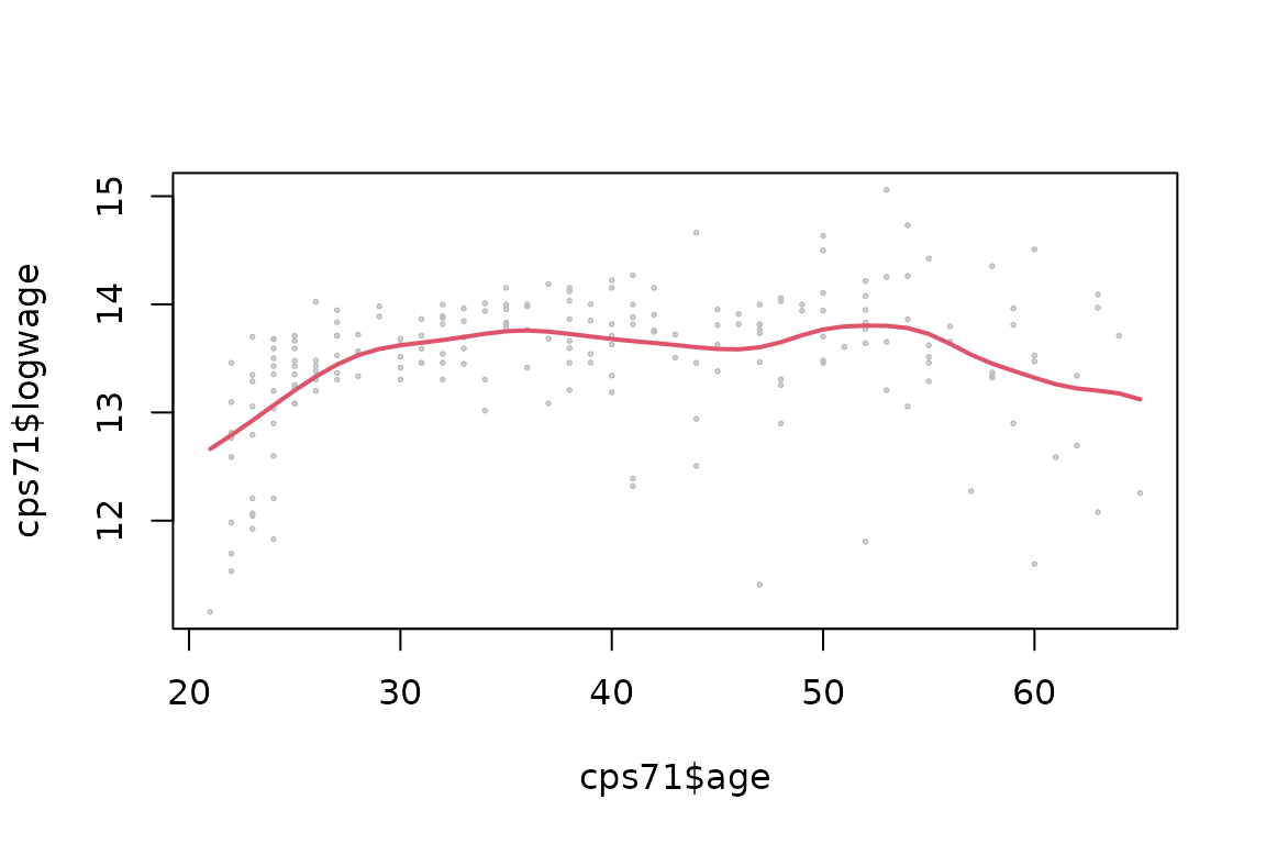
Mixed data
One important feature of np is that it handles mixed
data directly. Variable class matters: unordered categorical variables
should be factors, and ordered categorical variables should be ordered
factors when appropriate.
set.seed(42)
mydat <- data.frame(
  y = rnorm(200),
  x_cont = runif(200),
  x_unordered = factor(sample(c("a", "b", "c"), 200, replace = TRUE)),
  x_ordered = ordered(sample(1:4, 200, replace = TRUE))
)

bw_mixed <- npregbw(y ~ x_cont + x_unordered + x_ordered, data = mydat)
fit_mixed <- npreg(bws = bw_mixed)
summary(fit_mixed)
#>
#> Regression Data: 200 training points, in 3 variable(s)
#> Search Parameter(s):
#>          x_cont  x_unordered  x_ordered
#> Type  Bandwidth       Lambda     Lambda
#> Value   1729347    0.6610069  0.9981613
#> Max          --    0.6666667          1
#>
#> Kernel Regression Estimator: Local-Constant
#> Bandwidth Type: Fixed
#> Residual standard error: 0.9721457
#> R-squared: 0
#>
#> Continuous Kernel Type: Second-Order Gaussian
#> No. Continuous Explanatory Vars.: 1
#>
#> Unordered Categorical Kernel Type: Aitchison and Aitken
#> No. Unordered Categorical Explanatory Vars.: 1
#>
#> Ordered Categorical Kernel Type: Li and Racine
#> No. Ordered Categorical Explanatory Vars.: 1
#> Estimation Time: 0.454 seconds (optim 0.452s, fit 0.002s)
A note on modern local-polynomial search
For local-polynomial-capable methods, np now supports
joint selection of polynomial order and bandwidth. The modern route is
to use search.engine = "nomad+powell" when you want the
search to choose both together.
If you want the recommended route without spelling out all of the LP
tuning arguments, use nomad = TRUE. This is a documented
convenience preset, not a generic optimizer alias: it fills only missing
values among the LP degree-search controls and leaves compatible
explicit overrides in place. This route uses the optional NOMAD backend
provided by the suggested package crs, so install
crs first if you want to use nomad = TRUE or
search.engine = "nomad"/"nomad+powell".
if (requireNamespace("crs", quietly = TRUE) &&
    utils::packageVersion("crs") >= package_version("0.15-41")) {
  set.seed(7)
  n <- 120
  x <- runif(n, -1, 1)
  y <- x + 0.4 * x^2 + rnorm(n, sd = 0.18)

  fit_nomad <- npreg(y ~ x, nomad = TRUE, degree.max = 1L, nmulti = 1L)
  fit_nomad$bws$nomad.shortcut

  # Tune one component explicitly while leaving the rest of the preset in place.
  fit_nomad_direct <- npreg(
    y ~ x,
    nomad = TRUE,
    search.engine = "nomad",
    degree.max = 1L,
    nmulti = 1L
  )
}
The same convenience entry point is available for the other
LP-capable families: npcdens, npcdist,
npplreg, npscoef, and npindex,
together with their corresponding *bw constructors.
Keep the first run modest and runnable. Fuller worked examples belong on the gallery rather than in this package vignette.
Data preparation matters
In np, the formula interface tells the function which
variables are the response and regressors. It is not imposing an
ordinary linear-additive model.
It is also important not to pass blocks of 0/1 dummies as if this
were a standard linear-model workflow. If the underlying variable is
categorical, it is usually better to keep it as one factor
or ordered variable.
Other common starting points
This vignette keeps the package-side introduction intentionally narrow. Other common first routes are:
-
?npudensand?npudistfor unconditional density and distribution work, -
?npcdens,?npcdist, and?npqregfor conditional density, distribution, and quantiles, -
?npconmodefor classification and conditional mode estimation, -
?npplreg,?npindex, and?npscoeffor semiparametric models.
Those broader branches are better carried by help pages and website articles than by a single shipped vignette.
Where to go next
-
vignette("np_entropy_tests", package = "np")for a compact package-side testing overview -
?npreg,?npregbw,?npudens, and?npcdensfor core help pages - https://jeffreyracine.github.io/gallery/kernel_primer.html for the conceptual kernel overview
- https://jeffreyracine.github.io/gallery/density_distribution_quantiles.html for density, distribution, and quantile workflows
- https://jeffreyracine.github.io/gallery/semiparametric_models.html for partially linear, single-index, and varying-coefficient routes