01 - Introduction to ‘pbkrtest’

Søren Højsgaard and Ulrich Halekoh

## Loading required package: pbkrtest

## Loading required package: lme4

## Loading required package: Matrix

Package version: 0.5.4

Introduction

The data is a list of two vectors, giving the wear of shoes of materials A and B for one foot each of ten boys.

data(shoes, package="MASS")
shoes

## $A
##  [1] 13.2  8.2 10.9 14.3 10.7  6.6  9.5 10.8  8.8 13.3
## 
## $B
##  [1] 14.0  8.8 11.2 14.2 11.8  6.4  9.8 11.3  9.3 13.6

A plot reveals that boys wear their shoes differently.

plot(A ~ 1, data=shoes, col="red",lwd=2, pch=1, ylab="wear", xlab="boy")
points(B ~ 1, data=shoes, col="blue", lwd=2, pch=2)
points(I((A + B) / 2) ~ 1, data=shoes, pch="-", lwd=2)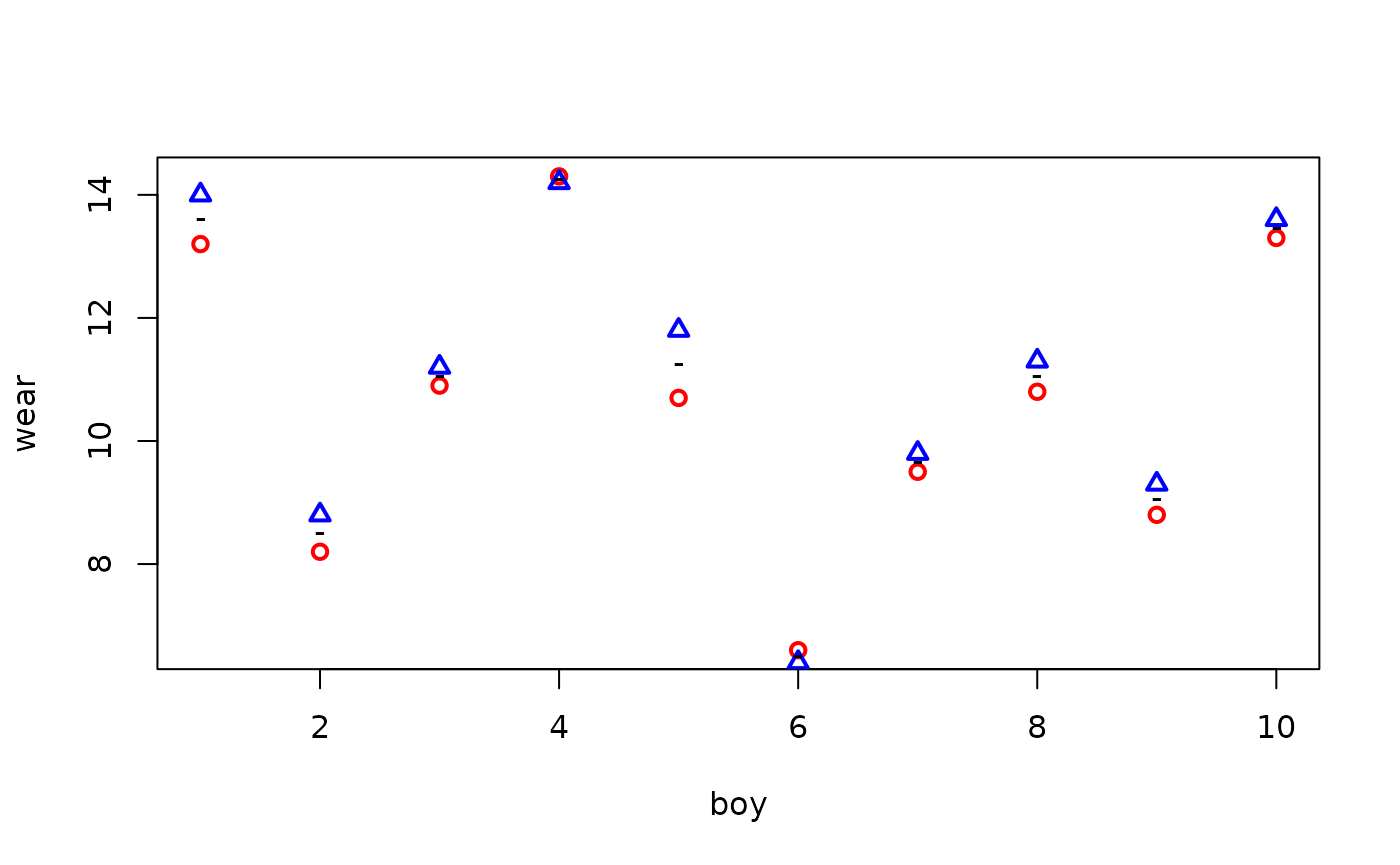

One option for testing the effect of materials is to make a paired $t$–test, e.g. as:

r1 <- t.test(shoes$A, shoes$B, paired=T)
r1 |> tidy()

## # A tibble: 1 × 8
##   estimate statistic p.value parameter conf.low conf.high method     alternative
##      <dbl>     <dbl>   <dbl>     <dbl>    <dbl>     <dbl> <chr>      <chr>      
## 1    -0.41     -3.35 0.00854         9   -0.687    -0.133 Paired t-… two.sided

To work with data in a mixed model setting we create a dataframe, and for later use we also create an imbalanced version of data:

boy <- rep(1:10, 2)
boyf<- factor(letters[boy])
material <- factor(c(rep("A", 10), rep("B", 10)))
## Balanced data:
shoe.bal <- data.frame(wear=unlist(shoes), boy=boy, boyf=boyf, material=material)
head(shoe.bal)

##    wear boy boyf material
## A1 13.2   1    a        A
## A2  8.2   2    b        A
## A3 10.9   3    c        A
## A4 14.3   4    d        A
## A5 10.7   5    e        A
## A6  6.6   6    f        A

## Imbalanced data; delete (boy=1, material=1) and (boy=2, material=b)
shoe.imbal <-  shoe.bal[-c(1, 12),]

We fit models to the two datasets:

lmm1.bal  <- lmer( wear ~ material + (1|boyf), data=shoe.bal)
lmm0.bal  <- update(lmm1.bal, .~. - material)
lmm1.imbal  <- lmer(wear ~ material + (1|boyf), data=shoe.imbal)
lmm0.imbal  <- update(lmm1.imbal, .~. - material)

The asymptotic likelihood ratio test shows stronger significance than the $t$–test:

anova(lmm1.bal, lmm0.bal, test="Chisq")  |> tidy()

## refitting model(s) with ML (instead of REML)

## # A tibble: 2 × 9
##   term      npar   AIC   BIC logLik minus2logL statistic    df  p.value
##   <chr>    <dbl> <dbl> <dbl>  <dbl>      <dbl>     <dbl> <dbl>    <dbl>
## 1 lmm0.bal     3  67.9  70.9  -31.0       61.9     NA       NA NA      
## 2 lmm1.bal     4  61.8  65.8  -26.9       53.8      8.09     1  0.00445

anova(lmm1.imbal, lmm0.imbal, test="Chisq")  |> tidy()

## refitting model(s) with ML (instead of REML)

## # A tibble: 2 × 9
##   term        npar   AIC   BIC logLik minus2logL statistic    df p.value
##   <chr>      <dbl> <dbl> <dbl>  <dbl>      <dbl>     <dbl> <dbl>   <dbl>
## 1 lmm0.imbal     3  63.9  66.5  -28.9       57.9     NA       NA NA     
## 2 lmm1.imbal     4  60.8  64.3  -26.4       52.8      5.09     1  0.0240

Kenward–Roger approach

The Kenward–Roger approximation is exact in certain balanced designs in the sense that the approximation produces the same result as the paired $t$–test.

kr.bal <- KRmodcomp(lmm1.bal, lmm0.bal)
kr.bal |> tidy()

## # A tibble: 1 × 5
##   term      stat    df   ddf p.value
##   <chr>    <dbl> <int> <dbl>   <dbl>
## 1 KR_Ftest  11.2     1  9.00 0.00854

summary(kr.bal) |> tidy() 

## # A tibble: 3 × 5
##   term       stat    df   ddf p.value
##   <chr>     <dbl> <int> <dbl>   <dbl>
## 1 LRT        8.12     1 NA    0.00438
## 2 KR_Ftest  11.2      1  9.00 0.00854
## 3 KR_FtestU 11.2      1  9.00 0.00854

For the imbalanced data we get

kr.imbal <- KRmodcomp(lmm1.imbal, lmm0.imbal)
kr.imbal |> tidy()

## # A tibble: 1 × 5
##   term      stat    df   ddf p.value
##   <chr>    <dbl> <int> <dbl>   <dbl>
## 1 KR_Ftest  5.99     1  7.02  0.0442

summary(kr.imbal) |> tidy()

## # A tibble: 3 × 5
##   term       stat    df   ddf p.value
##   <chr>     <dbl> <int> <dbl>   <dbl>
## 1 LRT        5.12     1 NA     0.0237
## 2 KR_Ftest   5.99     1  7.02  0.0442
## 3 KR_FtestU  5.99     1  7.02  0.0442

Notice that the Kenward-Roger approximation gives results similar to but not identical to the paired $t$–test when the two boys are removed:

shoes2 <- list(A=shoes$A[-(1:2)], B=shoes$B[-(1:2)])
t.test(shoes2$A, shoes2$B, paired=T) |> tidy()

## # A tibble: 1 × 8
##   estimate statistic p.value parameter conf.low conf.high method     alternative
##      <dbl>     <dbl>   <dbl>     <dbl>    <dbl>     <dbl> <chr>      <chr>      
## 1   -0.337     -2.39  0.0483         7   -0.672  -0.00328 Paired t-… two.sided

Satterthwaite approach

The Satterthwaite approximation is exact in certain balanced designs in the sense that the approximation produces the same result as the paired $t$–test.

sat.bal <- SATmodcomp(lmm1.bal, lmm0.bal)
sat.bal |> tidy()

## # A tibble: 1 × 5
##   term       stat    df   ddf p.value
##   <chr>     <dbl> <int> <dbl>   <dbl>
## 1 SAT_Ftest  11.2     1  9.00 0.00854

sat.imbal <- SATmodcomp(lmm1.imbal, lmm0.imbal)
sat.imbal |> tidy()

## # A tibble: 1 × 5
##   term       stat    df   ddf p.value
##   <chr>     <dbl> <int> <dbl>   <dbl>
## 1 SAT_Ftest  6.00     1  7.01  0.0441

Parametric bootstrap

Parametric bootstrap provides an alternative but many simulations are often needed to provide credible results (also many more than shown here; in this connection it can be useful to exploit that computations can be made en parallel, see the documentation):

pb.bal <- PBmodcomp(lmm1.bal, lmm0.bal, control=list(nsim=500, cl=2))
pb.bal |> tidy()

## # A tibble: 1 × 5
##   term    stat    df   ddf p.value
##   <chr>  <dbl> <dbl> <dbl>   <dbl>
## 1 PBtest  8.12    NA    NA 0.00399

summary(pb.bal) |> tidy()

## # A tibble: 3 × 5
##   term    stat    df   ddf  p.value
##   <chr>  <dbl> <dbl> <dbl>    <dbl>
## 1 LRT     8.12     1    NA  0.00438
## 2 PBtest  8.12    NA    NA  0.00399
## 3 NA     NA       NA    NA NA

For the imbalanced data, the result is similar to the result from the paired $t$–test.

pb.imbal <- PBmodcomp(lmm1.imbal, lmm0.imbal, control=list(nsim=500, cl=2))
pb.imbal |> tidy()

## # A tibble: 1 × 5
##   term    stat    df   ddf p.value
##   <chr>  <dbl> <dbl> <dbl>   <dbl>
## 1 PBtest  5.12    NA    NA  0.0659

summary(pb.imbal)  |> tidy()

## # A tibble: 3 × 5
##   term    stat    df   ddf p.value
##   <chr>  <dbl> <dbl> <dbl>   <dbl>
## 1 LRT     5.12     1    NA  0.0237
## 2 PBtest  5.12    NA    NA  0.0659
## 3 NA     NA       NA    NA NA

Matrices for random effects

The matrices involved in the random effects can be obtained with

shoe3 <- subset(shoe.bal, boy<=5)
shoe3 <- shoe3[order(shoe3$boy), ]
lmm1  <- lmer( wear ~ material + (1|boyf), data=shoe3 )
str( SG <- get_SigmaG( lmm1 ), max=2)

## List of 3
##  $ Sigma   :Formal class 'dgCMatrix' [package "Matrix"] with 6 slots
##  $ G       :List of 2
##   ..$ :Formal class 'dgCMatrix' [package "Matrix"] with 6 slots
##   ..$ :Formal class 'dgCMatrix' [package "Matrix"] with 6 slots
##  $ n.ggamma: int 2

round( SG$Sigma*10 )

## 10 x 10 sparse Matrix of class "dgCMatrix"

##   [[ suppressing 10 column names 'A1', 'B1', 'A2' ... ]]

##                                 
## A1 53 52  .  .  .  .  .  .  .  .
## B1 52 53  .  .  .  .  .  .  .  .
## A2  .  . 53 52  .  .  .  .  .  .
## B2  .  . 52 53  .  .  .  .  .  .
## A3  .  .  .  . 53 52  .  .  .  .
## B3  .  .  .  . 52 53  .  .  .  .
## A4  .  .  .  .  .  . 53 52  .  .
## B4  .  .  .  .  .  . 52 53  .  .
## A5  .  .  .  .  .  .  .  . 53 52
## B5  .  .  .  .  .  .  .  . 52 53

SG$G

## [[1]]
## 10 x 10 sparse Matrix of class "dgCMatrix"

##   [[ suppressing 10 column names 'A1', 'B1', 'A2' ... ]]

##                       
## A1 1 1 . . . . . . . .
## B1 1 1 . . . . . . . .
## A2 . . 1 1 . . . . . .
## B2 . . 1 1 . . . . . .
## A3 . . . . 1 1 . . . .
## B3 . . . . 1 1 . . . .
## A4 . . . . . . 1 1 . .
## B4 . . . . . . 1 1 . .
## A5 . . . . . . . . 1 1
## B5 . . . . . . . . 1 1
## 
## [[2]]
## 10 x 10 sparse Matrix of class "dgCMatrix"
##                          
##  [1,] 1 . . . . . . . . .
##  [2,] . 1 . . . . . . . .
##  [3,] . . 1 . . . . . . .
##  [4,] . . . 1 . . . . . .
##  [5,] . . . . 1 . . . . .
##  [6,] . . . . . 1 . . . .
##  [7,] . . . . . . 1 . . .
##  [8,] . . . . . . . 1 . .
##  [9,] . . . . . . . . 1 .
## [10,] . . . . . . . . . 1