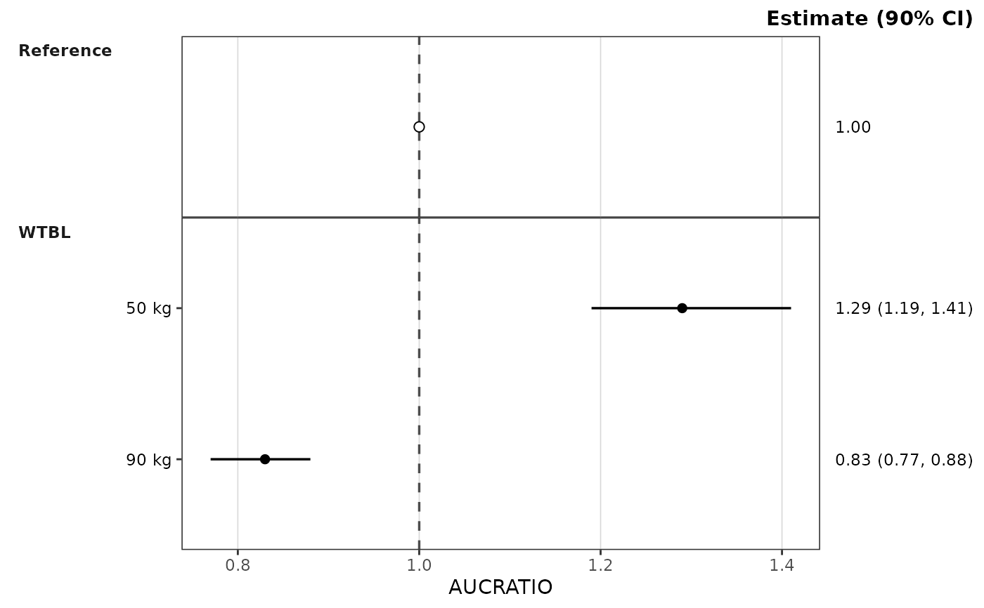
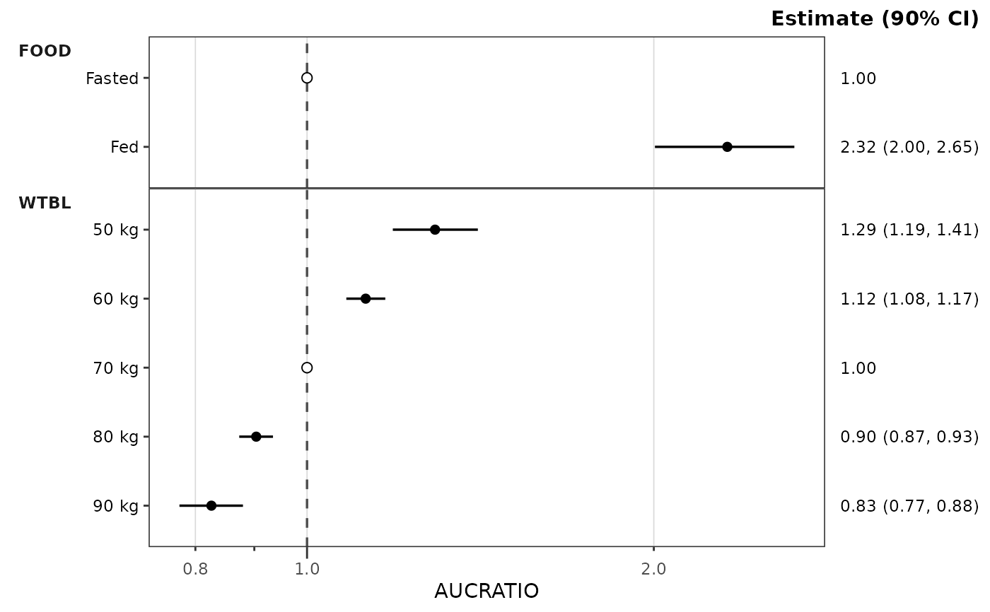
Build a forest plot ggplot from a forest_stats object

Constructs a covariate forest plot from a df_forest() result (or any object satisfying the forest_stats contract). Renders per-row point estimates with horizontal CI lines, optional shaded equivalence band, and a vertical reference line, one facet row per covariate name. The est_label, lo_label, and hi_label columns are assembled into the right-hand secondary y-axis text ("1.29 (1.19, 1.41)") under a header built from the container's ci (e.g. "Estimate (90% CI)"), so each row's estimate sits beside its point. The header is the plot subtitle, right-aligned so it sits on the top edge of the panels above the column; change it with + ggplot2::labs(subtitle = "Ratio (90% CI)"). The rendered metric labels the x-axis, and the plot has no title by default.

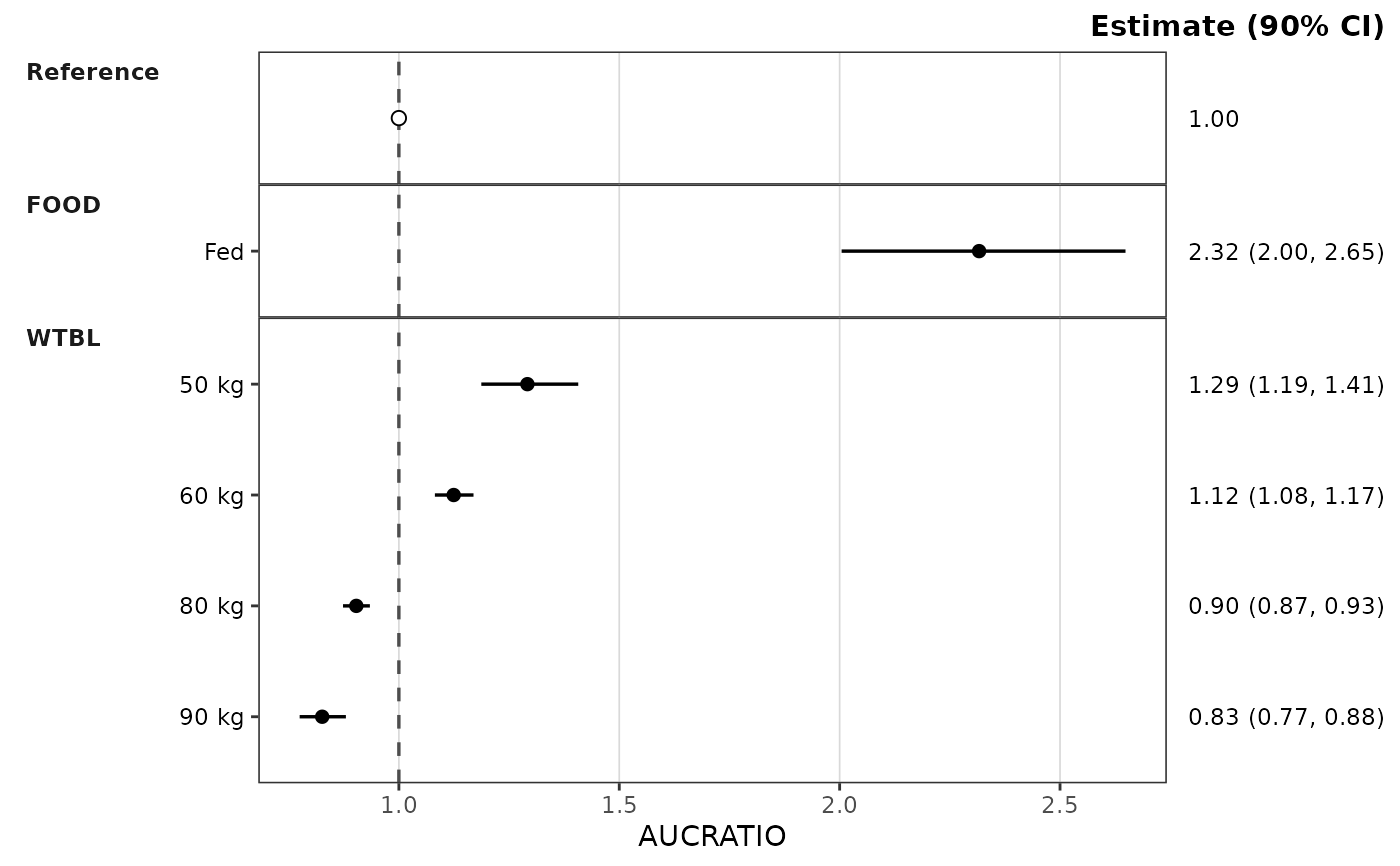
Rows are drawn in the order they appear in stats$stats, top to bottom (see the "Row order" section of df_forest()); reorder that frame to change the plot. Each row is its own y position, so covariate level labels may repeat across panels (Low / High under two covariates). The layout column selects the rows for the chosen reference layout (see ref_layout).

Rows flagged is_ref (the reference copies in each covariate panel, or the reference panel) draw through the ref_point style role (an open circle by default) and show the point estimate alone in the estimate column, since their CI collapses onto the estimate. A row whose level label repeats its covariate name (the reference panel) has no left-axis tick or label, since the strip already carries the name.

Returns a plain ggplot object so callers can compose additional layers, themes, and scales with the standard + operator.

Most users will reach this function indirectly via plot_forest(). Call plot_build_forest() directly when working from a manually- constructed or cached forest_stats object — for example, plotting a precomputed result from disk or a custom pipeline that produces compatible columns and config.

Usage

plot_build_forest(
  stats,
  metric = NULL,
  style = NULL,
  ref = "reference",
  ref_band = NULL,
  ref_band_type = c("multiplicative", "additive", "absolute"),
  ref_layout = NULL,
  show_rep = FALSE
)

Arguments

stats: A forest_stats object (typically the output of df_forest()), checked on entry; see "Building a forest_stats by hand" for the required columns and config.
metric: Character scalar identifying which value of metric_name_var to render. plot_forest() renders one metric per call (no metric facet); the covariate name is the only facet dimension. If NULL (default) and stats$stats contains exactly one unique value of metric_name_var, that value is used. If NULL and multiple metrics are present, aborts and asks the caller to pick one.
style: A ggstylekit::style_spec(); default style_forest(), which documents the roles, per-covariate coloring, and theme elements. Alternatives: style_forest_pmforest(), style_forest_coveffectsplot(), style_forest_pmxforest(), style_forest_pumas().
ref: The x-intercept of the vertical reference line: a numeric scalar, NULL to suppress the line, or "reference" (default) to use the estimate of the metric's reference row (the row flagged is_ref; exactly 1 for a ratio metric, the reference exposure for a raw metric). With "reference" and no reference row in the plotted metric, a warning is issued and no line is drawn.
ref_band: Length-2 increasing numeric vector (ref_band[1] < ref_band[2]) giving the equivalence band, read according to ref_band_type. Default NULL (no band).
ref_band_type: How ref_band is placed around the resolved ref: "multiplicative" (default) draws ref * ref_band, so c(0.8, 1.25) gives the bioequivalence bounds on a ratio or a raw exposure scale; "additive" draws ref + ref_band, so c(-10, 10) brackets a reference change of zero for a difference metric such as percent change from baseline; "absolute" draws ref_band as given. The first two require a resolved ref; multiplicative limits must be positive.
ref_layout: "distributed" draws the reference row inside each covariate panel named in cov_level_ref; "consolidated" draws it once in the reference panel at the top. Default NULL: distributed if df_forest() was given cov_level_ref for a covariate of metric, else consolidated.
show_rep: Logical. Display the number of replicates (the n column of the plotted rows) as a plot caption. Warns, and shows the range, when rows of the metric have different counts. Default FALSE. A caption set in the style is drawn instead, whatever this value.

Value

a ggplot plot object

Building a `forest_stats` by hand

Summaries computed elsewhere can be plotted by wrapping them with pmx_stats() and subclass = "forest_stats" (see the last example). stats needs one row per plotted point, in display order, with:

the metric, covariate name, and covariate level columns named in config (character);
est, lo, hi (numeric; the point and interval);
est_label, lo_label, hi_label (character; the plotted text) and ci_label (character; their combined form);
is_ref (logical, no NA; the reference rows);
layout: "both" for covariate rows, "consolidated" for a reference-panel row, "distributed" for a reference copy inside a covariate panel;
optionally n (integer draw count), needed only for show_rep.

config needs metric_name_var, cov_name_var, and cov_level_var (the column names), ci (in (0, 1), used in the header), and sigdigits (a whole number >= 1). The object is checked when plotted.

Examples

stats <- df_forest(
  data_sad_pkforest,
  cov_level_ref = attr(data_sad_pkforest, "cov_level_ref")
)
plot_build_forest(stats, metric = "AUCRATIO")

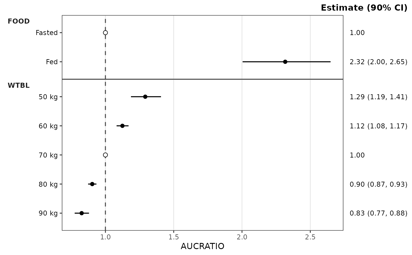plot_build_forest(stats, metric = "AUCRATIO", ref_band = c(0.8, 1.25))

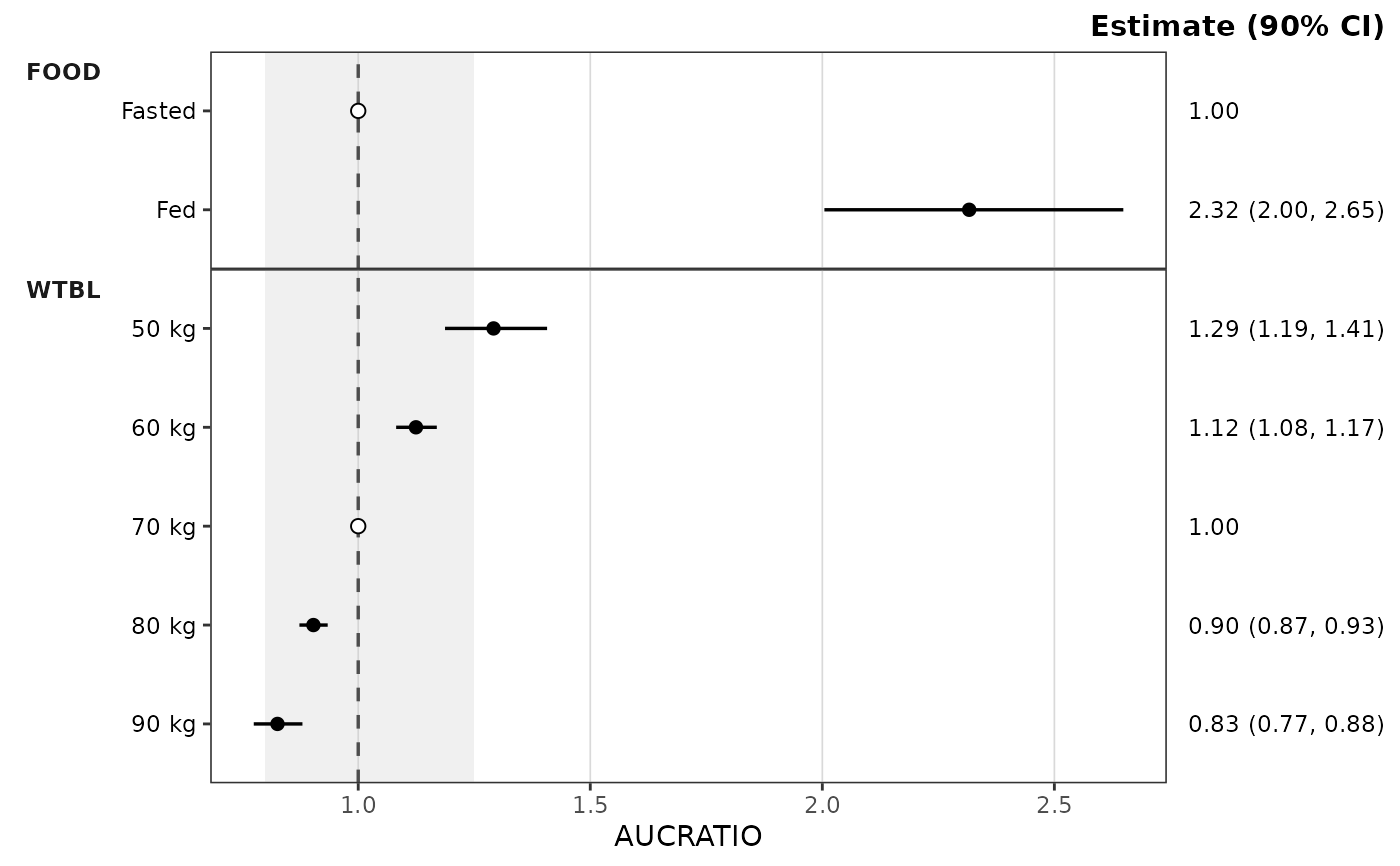# The same stats with the reference panel
plot_build_forest(stats, metric = "AUCRATIO", ref_layout = "consolidated")

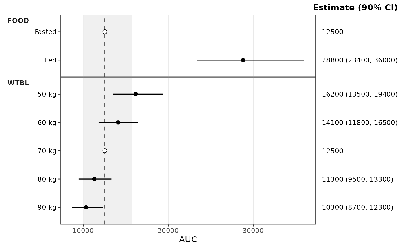
# Raw exposure: the line sits at the reference exposure and the band is
# 0.8 to 1.25 times it
plot_build_forest(stats, metric = "AUC", ref_band = c(0.8, 1.25))

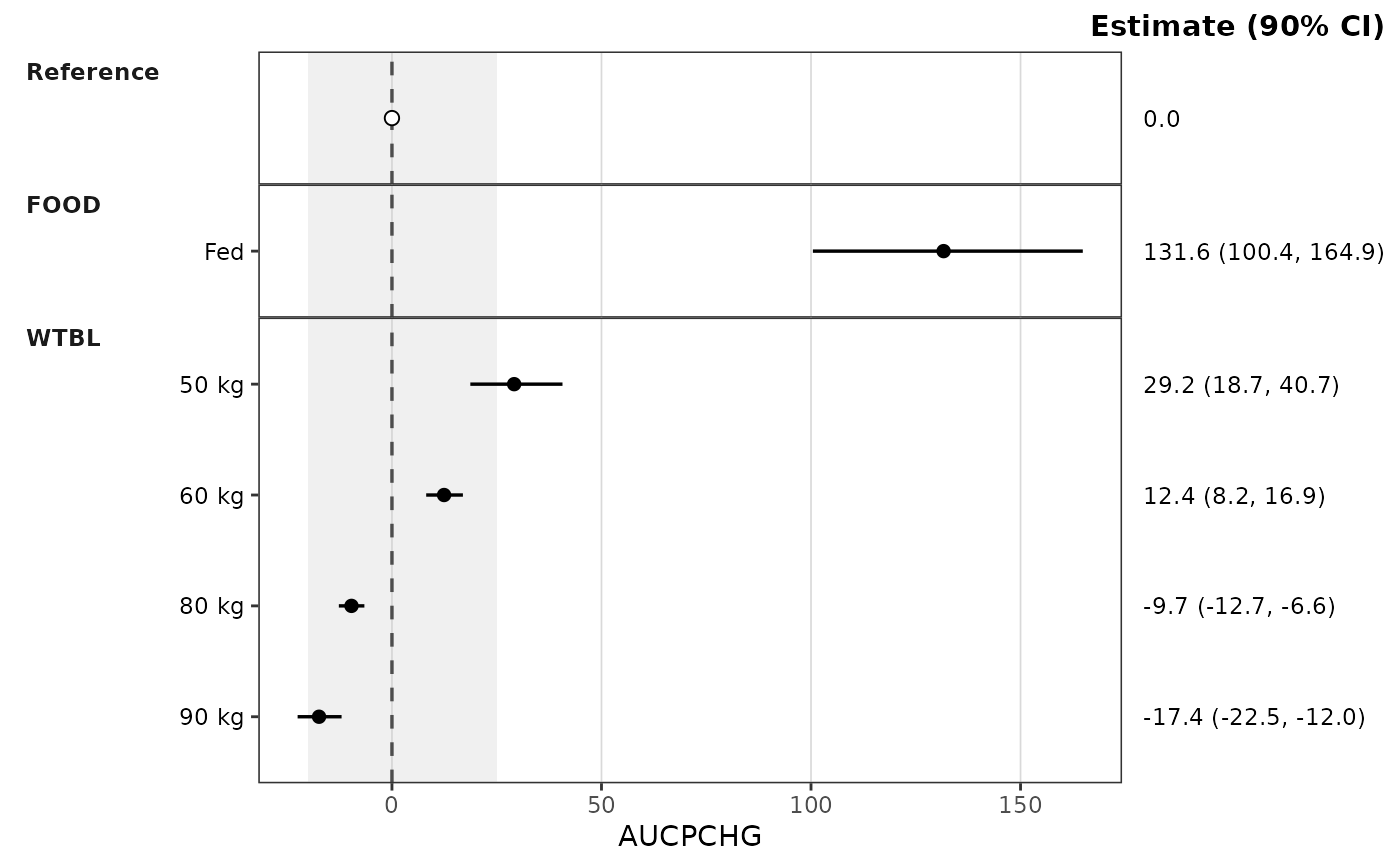
# Difference metric: percent change from the reference, with an additive
# band around the reference change of 0
pchg <- dplyr::filter(data_sad_pkforest, metric == "AUCRATIO") |>
  dplyr::mutate(metric = "AUCPCHG", value = 100 * (value - 1))
plot_build_forest(df_forest(pchg), ref_band = c(-20, 25),
                  ref_band_type = "additive")

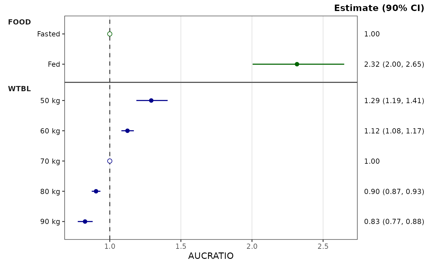
# Per-covariate coloring via the style's `colors` map
plot_build_forest(
  stats, metric = "AUCRATIO",
  style = style_forest(colors = c(FOOD = "darkgreen", WTBL = "darkblue"))
)

# Log x-axis: through the style, or compose with ggplot2 directly
plot_build_forest(stats, metric = "AUCRATIO", style = style_forest(logx = TRUE))

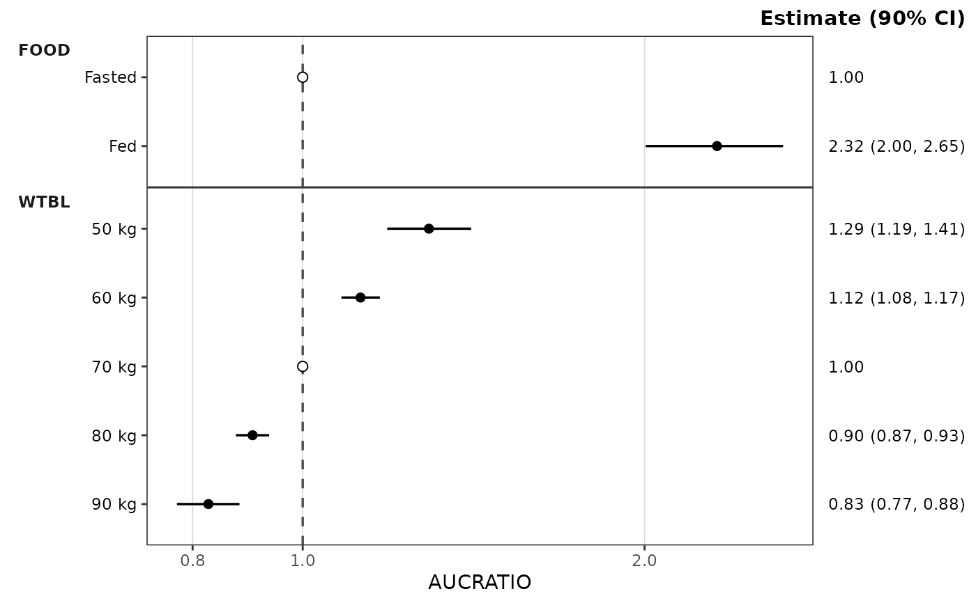plot_build_forest(stats, metric = "AUCRATIO") +
  ggplot2::scale_x_log10(guide = "axis_logticks")

# A summary built by hand
manual <- pmx_stats(
  stats = data.frame(
    metric = "AUCRATIO",
    cov_name = c("Reference", "WTBL", "WTBL"),
    cov_level = c("Reference", "50 kg", "90 kg"),
    est = c(1, 1.29, 0.83), lo = c(1, 1.19, 0.77), hi = c(1, 1.41, 0.88),
    est_label = c("1.00", "1.29", "0.83"),
    lo_label = c("1.00", "1.19", "0.77"),
    hi_label = c("1.00", "1.41", "0.88"),
    ci_label = c("1.00 (1.00, 1.00)", "1.29 (1.19, 1.41)", "0.83 (0.77, 0.88)"),
    is_ref = c(TRUE, FALSE, FALSE),
    layout = c("consolidated", "both", "both")
  ),
  config = list(metric_name_var = "metric", cov_name_var = "cov_name",
                cov_level_var = "cov_level", ci = 0.9, sigdigits = 3),
  subclass = "forest_stats"
)
plot_build_forest(manual)