Classification and Regression with Random Forest

randomForest implements Breiman's random forest algorithm (based on Breiman and Cutler's original Fortran code) for classification and regression. It can also be used in unsupervised mode for assessing proximities among data points.

# S3 method for class 'formula'
randomForest(formula, data=NULL, ..., subset, na.action=na.fail)
# Default S3 method
randomForest(x, y=NULL,  xtest=NULL, ytest=NULL, ntree=500,
             mtry=if (!is.null(y) && !is.factor(y))
             max(floor(ncol(x)/3), 1) else floor(sqrt(ncol(x))),
             weights=NULL,
             replace=TRUE, classwt=NULL, cutoff, strata,
             sampsize = if (replace) nrow(x) else ceiling(.632*nrow(x)),
             nodesize = if (!is.null(y) && !is.factor(y)) 5 else 1,
             maxnodes = NULL,
             importance=FALSE, localImp=FALSE, nPerm=1,
             proximity, oob.prox=proximity,
             norm.votes=TRUE, do.trace=FALSE,
             keep.forest=!is.null(y) && is.null(xtest), corr.bias=FALSE,
             keep.inbag=FALSE, ...)
# S3 method for class 'randomForest'
print(x, ...)

Arguments

data: an optional data frame containing the variables in the model. By default the variables are taken from the environment which randomForest is called from.
subset: an index vector indicating which rows should be used. (NOTE: If given, this argument must be named.)
na.action: A function to specify the action to be taken if NAs are found. (NOTE: If given, this argument must be named.)
x, formula: a data frame or a matrix of predictors, or a formula describing the model to be fitted (for the print method, an randomForest object).
y: A response vector. If a factor, classification is assumed, otherwise regression is assumed. If omitted, randomForest will run in unsupervised mode.
xtest: a data frame or matrix (like x) containing predictors for the test set.
ytest: response for the test set.
ntree: Number of trees to grow. This should not be set to too small a number, to ensure that every input row gets predicted at least a few times.
mtry: Number of variables randomly sampled as candidates at each split. Note that the default values are different for classification (sqrt(p) where p is number of variables in x) and regression (p/3)
weights: A vector of length same as y that are positive weights used only in sampling data to grow each tree (not used in any other calculation)
replace: Should sampling of cases be done with or without replacement?
classwt: Priors of the classes. Need not add up to one. Ignored for regression.
cutoff: (Classification only) A vector of length equal to number of classes. The `winning' class for an observation is the one with the maximum ratio of proportion of votes to cutoff. Default is 1/k where k is the number of classes (i.e., majority vote wins).
strata: A (factor) variable that is used for stratified sampling.
sampsize: Size(s) of sample to draw. For classification, if sampsize is a vector of the length the number of strata, then sampling is stratified by strata, and the elements of sampsize indicate the numbers to be drawn from the strata.
nodesize: Minimum size of terminal nodes. Setting this number larger causes smaller trees to be grown (and thus take less time). Note that the default values are different for classification (1) and regression (5).
maxnodes: Maximum number of terminal nodes trees in the forest can have. If not given, trees are grown to the maximum possible (subject to limits by nodesize). If set larger than maximum possible, a warning is issued.
importance: Should importance of predictors be assessed?
localImp: Should casewise importance measure be computed? (Setting this to TRUE will override importance.)
nPerm: Number of times the OOB data are permuted per tree for assessing variable importance. Number larger than 1 gives slightly more stable estimate, but not very effective. Currently only implemented for regression.
proximity: Should proximity measure among the rows be calculated?
oob.prox: Should proximity be calculated only on “out-of-bag” data?
norm.votes: If TRUE (default), the final result of votes are expressed as fractions. If FALSE, raw vote counts are returned (useful for combining results from different runs). Ignored for regression.
do.trace: If set to TRUE, give a more verbose output as randomForest is run. If set to some integer, then running output is printed for every do.trace trees.
keep.forest: If set to FALSE, the forest will not be retained in the output object. If xtest is given, defaults to FALSE.
corr.bias: perform bias correction for regression? Note: Experimental. Use at your own risk.
keep.inbag: Should an n by ntree matrix be returned that keeps track of which samples are “in-bag” in which trees (but not how many times, if sampling with replacement)
...: optional parameters to be passed to the low level function randomForest.default.

Value

An object of class randomForest, which is a list with the following components:

call: the original call to randomForest
type: one of regression, classification, or unsupervised.
predicted: the predicted values of the input data based on out-of-bag samples.
importance: a matrix with nclass + 2 (for classification) or two (for regression) columns. For classification, the first nclass columns are the class-specific measures computed as mean descrease in accuracy. The nclass + 1st column is the mean descrease in accuracy over all classes. The last column is the mean decrease in Gini index. For Regression, the first column is the mean decrease in accuracy and the second the mean decrease in MSE. If importance=FALSE, the last measure is still returned as a vector.
importanceSD: The “standard errors” of the permutation-based importance measure. For classification, a p by nclass + 1 matrix corresponding to the first nclass + 1 columns of the importance matrix. For regression, a length p vector.
localImp: a p by n matrix containing the casewise importance measures, the [i,j] element of which is the importance of i-th variable on the j-th case. NULL if localImp=FALSE.
ntree: number of trees grown.
mtry: number of predictors sampled for spliting at each node.
forest: (a list that contains the entire forest; NULL if randomForest is run in unsupervised mode or if keep.forest=FALSE.
err.rate: (classification only) vector error rates of the prediction on the input data, the i-th element being the (OOB) error rate for all trees up to the i-th.
confusion: (classification only) the confusion matrix of the prediction (based on OOB data).
votes: (classification only) a matrix with one row for each input data point and one column for each class, giving the fraction or number of (OOB) `votes' from the random forest.
oob.times: number of times cases are `out-of-bag' (and thus used in computing OOB error estimate)
proximity: if proximity=TRUE when randomForest is called, a matrix of proximity measures among the input (based on the frequency that pairs of data points are in the same terminal nodes).
mse: (regression only) vector of mean square errors: sum of squared residuals divided by n.
rsq: (regression only) “pseudo R-squared”: 1 - mse / Var(y).
test: if test set is given (through the xtest or additionally ytest arguments), this component is a list which contains the corresponding predicted, err.rate, confusion, votes (for classification) or predicted, mse and rsq (for regression) for the test set. If proximity=TRUE, there is also a component, proximity, which contains the proximity among the test set as well as proximity between test and training data.

Note

The forest structure is slightly different between classification and regression. For details on how the trees are stored, see the help page for getTree.

If xtest is given, prediction of the test set is done “in place” as the trees are grown. If ytest is also given, and do.trace is set to some positive integer, then for every do.trace trees, the test set error is printed. Results for the test set is returned in the test component of the resulting randomForest object. For classification, the votes component (for training or test set data) contain the votes the cases received for the classes. If norm.votes=TRUE, the fraction is given, which can be taken as predicted probabilities for the classes.

For large data sets, especially those with large number of variables, calling randomForest via the formula interface is not advised: There may be too much overhead in handling the formula.

The “local” (or casewise) variable importance is computed as follows: For classification, it is the increase in percent of times a case is OOB and misclassified when the variable is permuted. For regression, it is the average increase in squared OOB residuals when the variable is permuted.

References

Breiman, L. (2001), Random Forests, Machine Learning 45(1), 5-32.

Breiman, L (2002), “Manual On Setting Up, Using, And Understanding Random Forests V3.1”, https://www.stat.berkeley.edu/~breiman/Using_random_forests_V3.1.pdf.

Author

Andy Liaw andy_liaw@merck.com and Matthew Wiener matthew_wiener@merck.com, based on original Fortran code by Leo Breiman and Adele Cutler.

Examples

## Classification:
##data(iris)
set.seed(71)
iris.rf <- randomForest(Species ~ ., data=iris, importance=TRUE,
                        proximity=TRUE)
print(iris.rf)
#> 
#> Call:
#>  randomForest(formula = Species ~ ., data = iris, importance = TRUE,      proximity = TRUE) 
#>                Type of random forest: classification
#>                      Number of trees: 500
#> No. of variables tried at each split: 2
#> 
#>         OOB estimate of  error rate: 4.67%
#> Confusion matrix:
#>            setosa versicolor virginica class.error
#> setosa         50          0         0        0.00
#> versicolor      0         47         3        0.06
#> virginica       0          4        46        0.08
## Look at variable importance:
round(importance(iris.rf), 2)
#>              setosa versicolor virginica MeanDecreaseAccuracy MeanDecreaseGini
#> Sepal.Length   5.88       5.87      9.21                10.62             9.37
#> Sepal.Width    5.23       0.31      4.71                 4.94             2.45
#> Petal.Length  21.60      31.41     27.71                32.39            42.13
#> Petal.Width   22.96      33.74     32.07                33.85            45.28
## Do MDS on 1 - proximity:
iris.mds <- cmdscale(1 - iris.rf$proximity, eig=TRUE)
op <- par(pty="s")
pairs(cbind(iris[,1:4], iris.mds$points), cex=0.6, gap=0,
      col=c("red", "green", "blue")[as.numeric(iris$Species)],
      main="Iris Data: Predictors and MDS of Proximity Based on RandomForest")

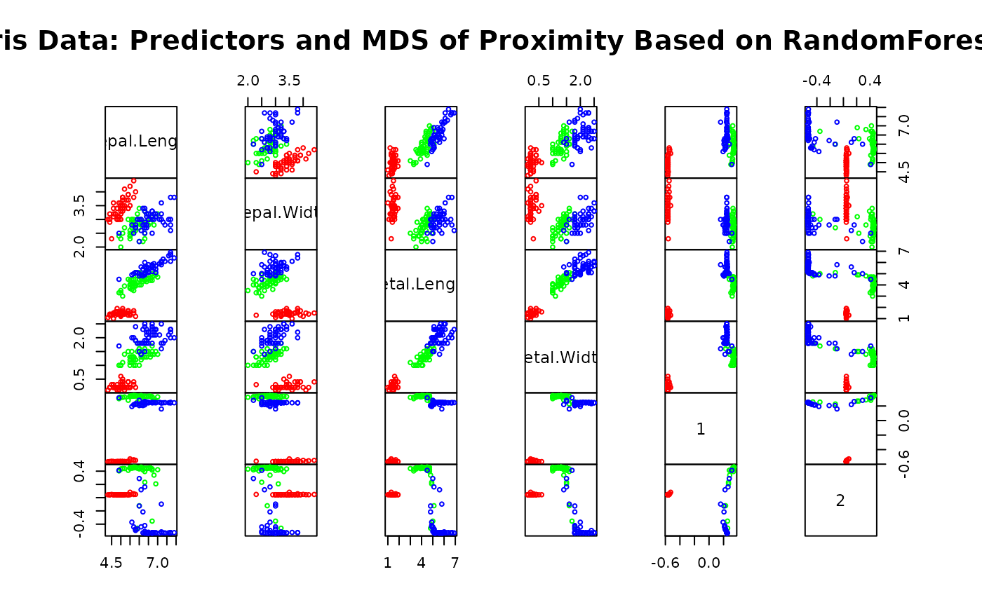par(op)
print(iris.mds$GOF)
#> [1] 0.7373483 0.7989356

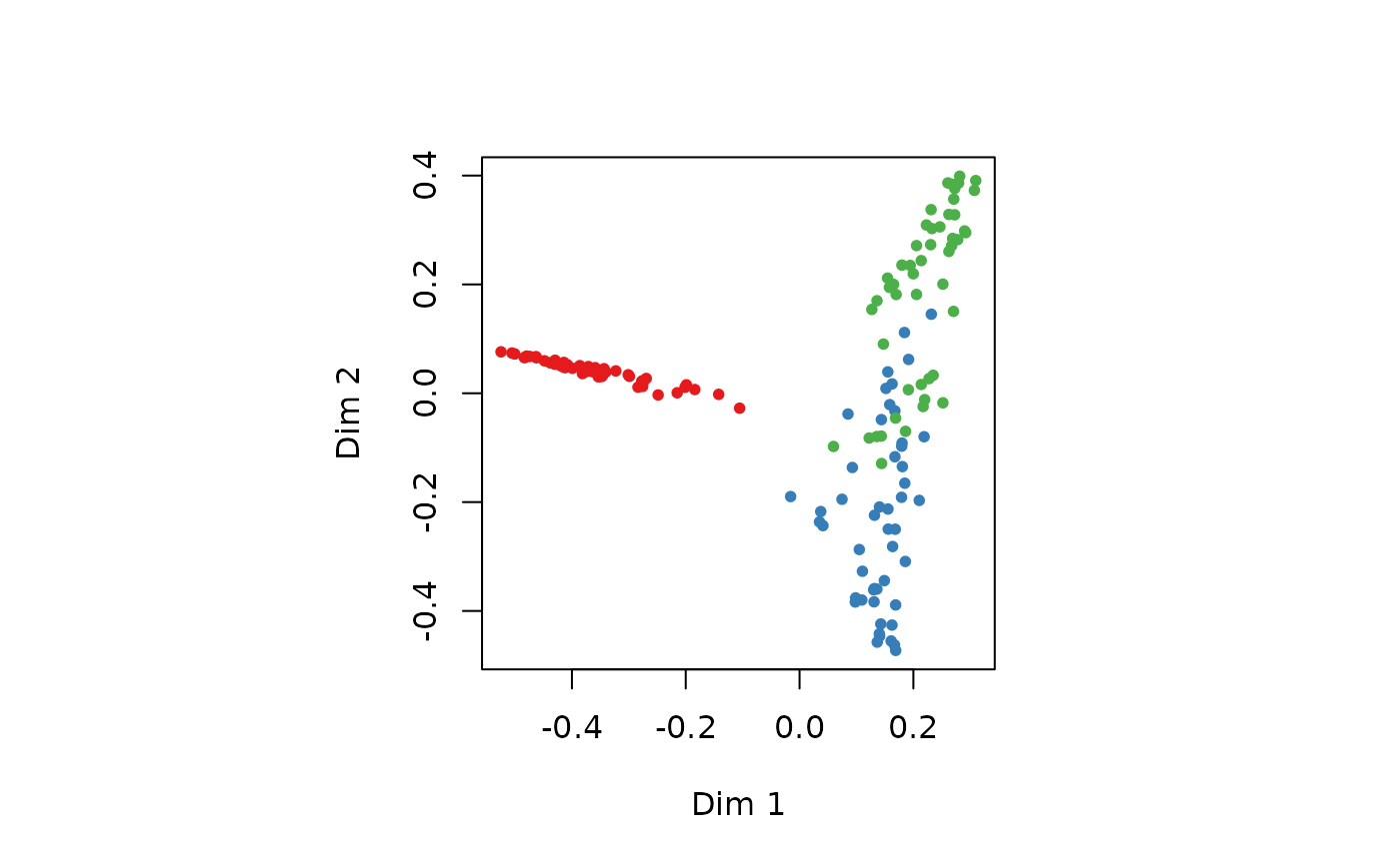
## The `unsupervised' case:
set.seed(17)
iris.urf <- randomForest(iris[, -5])
MDSplot(iris.urf, iris$Species)


## stratified sampling: draw 20, 30, and 20 of the species to grow each tree.
(iris.rf2 <- randomForest(iris[1:4], iris$Species, 
                          sampsize=c(20, 30, 20)))
#> 
#> Call:
#>  randomForest(x = iris[1:4], y = iris$Species, sampsize = c(20,      30, 20)) 
#>                Type of random forest: classification
#>                      Number of trees: 500
#> No. of variables tried at each split: 2
#> 
#>         OOB estimate of  error rate: 4.67%
#> Confusion matrix:
#>            setosa versicolor virginica class.error
#> setosa         50          0         0        0.00
#> versicolor      0         47         3        0.06
#> virginica       0          4        46        0.08

## Regression:
## data(airquality)
set.seed(131)
ozone.rf <- randomForest(Ozone ~ ., data=airquality, mtry=3,
                         importance=TRUE, na.action=na.omit)
print(ozone.rf)
#> 
#> Call:
#>  randomForest(formula = Ozone ~ ., data = airquality, mtry = 3,      importance = TRUE, na.action = na.omit) 
#>                Type of random forest: regression
#>                      Number of trees: 500
#> No. of variables tried at each split: 3
#> 
#>           Mean of squared residuals: 302.2117
#>                     % Var explained: 72.46
## Show "importance" of variables: higher value mean more important:
round(importance(ozone.rf), 2)
#>         %IncMSE IncNodePurity
#> Solar.R    9.76      10741.33
#> Wind      22.15      44234.96
#> Temp      43.85      53787.56
#> Month      2.59       1692.48
#> Day        0.93       6606.39

## "x" can be a matrix instead of a data frame:
set.seed(17)
x <- matrix(runif(5e2), 100)
y <- gl(2, 50)
(myrf <- randomForest(x, y))
#> 
#> Call:
#>  randomForest(x = x, y = y) 
#>                Type of random forest: classification
#>                      Number of trees: 500
#> No. of variables tried at each split: 2
#> 
#>         OOB estimate of  error rate: 52%
#> Confusion matrix:
#>    1  2 class.error
#> 1 25 25        0.50
#> 2 27 23        0.54
(predict(myrf, x))
#>   1   2   3   4   5   6   7   8   9  10  11  12  13  14  15  16  17  18  19  20 
#>   1   1   1   1   1   1   1   1   1   1   1   1   1   1   1   1   1   1   1   1 
#>  21  22  23  24  25  26  27  28  29  30  31  32  33  34  35  36  37  38  39  40 
#>   1   1   1   1   1   1   1   1   1   1   1   1   1   1   1   1   1   1   1   1 
#>  41  42  43  44  45  46  47  48  49  50  51  52  53  54  55  56  57  58  59  60 
#>   1   1   1   1   1   1   1   1   1   1   2   2   2   2   2   2   2   2   2   2 
#>  61  62  63  64  65  66  67  68  69  70  71  72  73  74  75  76  77  78  79  80 
#>   2   2   2   2   2   2   2   2   2   2   2   2   2   2   2   2   2   2   2   2 
#>  81  82  83  84  85  86  87  88  89  90  91  92  93  94  95  96  97  98  99 100 
#>   2   2   2   2   2   2   2   2   2   2   2   2   2   2   2   2   2   2   2   2 
#> Levels: 1 2

## "complicated" formula:
(swiss.rf <- randomForest(sqrt(Fertility) ~ . - Catholic + I(Catholic < 50),
                          data=swiss))
#> 
#> Call:
#>  randomForest(formula = sqrt(Fertility) ~ . - Catholic + I(Catholic <      50), data = swiss) 
#>                Type of random forest: regression
#>                      Number of trees: 500
#> No. of variables tried at each split: 1
#> 
#>           Mean of squared residuals: 0.3277816
#>                     % Var explained: 44.34
(predict(swiss.rf, swiss))
#>   Courtelary     Delemont Franches-Mnt      Moutier   Neuveville   Porrentruy 
#>     8.541742     8.992064     9.124838     8.760460     8.541086     8.949770 
#>        Broye        Glane      Gruyere       Sarine      Veveyse        Aigle 
#>     8.933005     9.149158     8.908574     8.887482     9.117942     7.922911 
#>      Aubonne     Avenches     Cossonay    Echallens     Grandson     Lausanne 
#>     8.333468     8.221398     8.031662     8.306702     8.439164     7.720665 
#>    La Vallee       Lavaux       Morges       Moudon        Nyone         Orbe 
#>     7.571783     8.193442     7.984520     8.340828     7.854661     7.872754 
#>         Oron      Payerne Paysd'enhaut        Rolle        Vevey      Yverdon 
#>     8.497338     8.503535     8.411120     8.035106     7.839470     8.330708 
#>      Conthey    Entremont       Herens     Martigwy      Monthey   St Maurice 
#>     8.834288     8.654145     8.757652     8.560958     8.882983     8.469376 
#>       Sierre         Sion       Boudry La Chauxdfnd     Le Locle    Neuchatel 
#>     8.928218     8.635219     8.258310     8.028697     8.177889     7.779149 
#>   Val de Ruz ValdeTravers V. De Geneve  Rive Droite  Rive Gauche 
#>     8.573018     8.155001     6.776675     7.527191     7.289894 
## Test use of 32-level factor as a predictor:
set.seed(1)
x <- data.frame(x1=gl(53, 10), x2=runif(530), y=rnorm(530))
(rf1 <- randomForest(x[-3], x[[3]], ntree=10))
#> 
#> Call:
#>  randomForest(x = x[-3], y = x[[3]], ntree = 10) 
#>                Type of random forest: regression
#>                      Number of trees: 10
#> No. of variables tried at each split: 1
#> 
#>           Mean of squared residuals: 1.599315
#>                     % Var explained: -44.33

## Grow no more than 4 nodes per tree:
(treesize(randomForest(Species ~ ., data=iris, maxnodes=4, ntree=30)))
#>  [1] 4 4 4 4 4 4 4 4 4 4 4 4 4 4 4 4 4 4 4 4 4 4 4 4 4 4 4 4 4 4

## test proximity in regression
iris.rrf <- randomForest(iris[-1], iris[[1]], ntree=101, proximity=TRUE, oob.prox=FALSE)
str(iris.rrf$proximity)
#>  num [1:150, 1:150] 1 0.386 0.347 0.307 0.881 ...
#>  - attr(*, "dimnames")=List of 2
#>   ..$ : chr [1:150] "1" "2" "3" "4" ...
#>   ..$ : chr [1:150] "1" "2" "3" "4" ...

## Using weights: make versicolors having 3 times larger weights
iris_wt <- ifelse( iris$Species == "versicolor", 3, 1 )
set.seed(15)
iris.wcrf <- randomForest(iris[-5], iris[[5]], weights=iris_wt, keep.inbag=TRUE)
print(rowSums(iris.wcrf$inbag))
#>   1   2   3   4   5   6   7   8   9  10  11  12  13  14  15  16  17  18  19  20 
#> 321 316 314 322 320 266 302 296 275 294 294 280 286 312 307 291 285 296 292 316 
#>  21  22  23  24  25  26  27  28  29  30  31  32  33  34  35  36  37  38  39  40 
#> 312 286 287 258 310 289 271 287 300 319 286 311 289 296 292 294 291 305 281 293 
#>  41  42  43  44  45  46  47  48  49  50  51  52  53  54  55  56  57  58  59  60 
#> 296 294 305 270 340 300 282 311 283 301 888 912 905 874 921 908 899 954 925 933 
#>  61  62  63  64  65  66  67  68  69  70  71  72  73  74  75  76  77  78  79  80 
#> 927 906 927 927 941 901 881 934 913 917 910 885 869 904 957 861 878 896 908 936 
#>  81  82  83  84  85  86  87  88  89  90  91  92  93  94  95  96  97  98  99 100 
#> 871 902 879 883 926 905 906 835 890 895 915 902 877 918 974 905 900 889 884 910 
#> 101 102 103 104 105 106 107 108 109 110 111 112 113 114 115 116 117 118 119 120 
#> 301 306 287 319 323 278 277 288 315 286 303 277 284 295 312 325 267 312 298 333 
#> 121 122 123 124 125 126 127 128 129 130 131 132 133 134 135 136 137 138 139 140 
#> 308 300 306 303 311 301 303 301 287 308 284 296 309 260 291 325 281 272 281 287 
#> 141 142 143 144 145 146 147 148 149 150 
#> 305 318 295 328 307 274 341 276 304 265 
set.seed(15)
iris.wrrf <- randomForest(iris[-1], iris[[1]], weights=iris_wt, keep.inbag=TRUE)
print(rowSums(iris.wrrf$inbag))
#>   1   2   3   4   5   6   7   8   9  10  11  12  13  14  15  16  17  18  19  20 
#> 292 308 324 302 276 290 331 325 290 306 297 298 289 286 293 295 308 296 304 324 
#>  21  22  23  24  25  26  27  28  29  30  31  32  33  34  35  36  37  38  39  40 
#> 286 275 307 263 317 287 275 288 297 303 272 294 298 287 267 275 296 263 310 295 
#>  41  42  43  44  45  46  47  48  49  50  51  52  53  54  55  56  57  58  59  60 
#> 332 303 315 274 303 303 311 279 278 282 862 901 903 847 882 896 863 924 890 901 
#>  61  62  63  64  65  66  67  68  69  70  71  72  73  74  75  76  77  78  79  80 
#> 945 925 930 872 917 903 903 907 904 885 916 898 917 862 958 916 906 901 884 861 
#>  81  82  83  84  85  86  87  88  89  90  91  92  93  94  95  96  97  98  99 100 
#> 895 914 909 900 896 894 893 875 872 928 904 950 900 952 935 878 912 942 929 945 
#> 101 102 103 104 105 106 107 108 109 110 111 112 113 114 115 116 117 118 119 120 
#> 285 300 306 312 310 315 302 287 277 279 302 301 298 292 295 306 285 319 304 294 
#> 121 122 123 124 125 126 127 128 129 130 131 132 133 134 135 136 137 138 139 140 
#> 323 294 309 315 297 273 297 300 299 289 285 289 317 311 310 350 290 305 312 315 
#> 141 142 143 144 145 146 147 148 149 150 
#> 268 338 289 332 293 290 324 264 310 272