Polynomial kernel PCA signal extraction

step_kpca_poly() creates a specification of a recipe step that will convert numeric data into one or more principal components using a polynomial kernel basis expansion.

step_kpca_poly(
  recipe,
  ...,
  role = "predictor",
  trained = FALSE,
  num_comp = 5,
  res = NULL,
  columns = NULL,
  degree = 2,
  scale_factor = 1,
  offset = 1,
  prefix = "kPC",
  keep_original_cols = FALSE,
  skip = FALSE,
  id = rand_id("kpca_poly")
)

Arguments

recipe

A recipe object. The step will be added to the sequence of operations for this recipe.

...

One or more selector functions to choose variables for this step. See selections() for more details.

role

For model terms created by this step, what analysis role should they be assigned? By default, the new columns created by this step from the original variables will be used as predictors in a model.

trained

A logical to indicate if the quantities for preprocessing have been estimated.

num_comp

The number of components to retain as new predictors. If num_comp is greater than the number of columns or the number of possible components, a smaller value will be used. If num_comp = 0 is set then no transformation is done and selected variables will stay unchanged, regardless of the value of keep_original_cols.

res

An S4 kernlab::kpca() object is stored here once this preprocessing step has be trained by prep().

columns

A character string of the selected variable names. This field is a placeholder and will be populated once prep() is used.

degree, scale_factor, offset

Numeric values for the polynomial kernel function. See the documentation at kernlab::polydot().

prefix

A character string for the prefix of the resulting new variables. See notes below.

keep_original_cols

A logical to keep the original variables in the output. Defaults to FALSE.

skip

A logical. Should the step be skipped when the recipe is baked by bake()? While all operations are baked when prep() is run, some operations may not be able to be conducted on new data (e.g. processing the outcome variable(s)). Care should be taken when using skip = TRUE as it may affect the computations for subsequent operations.

id

A character string that is unique to this step to identify it.

Value

An updated version of recipe with the new step added to the sequence of any existing operations.

Details

Kernel principal component analysis (kPCA) is an extension of a PCA analysis that conducts the calculations in a broader dimensionality defined by a kernel function. For example, if a quadratic kernel function were used, each variable would be represented by its original values as well as its square. This nonlinear mapping is used during the PCA analysis and can potentially help find better representations of the original data.

This step requires the kernlab package. If not installed, the step will stop with a prompt about installing the package.

As with ordinary PCA, it is important to center and scale the variables prior to computing PCA components (step_normalize() can be used for this purpose).

The argument num_comp controls the number of components that will be retained (the original variables that are used to derive the components are removed from the data). The new components will have names that begin with prefix and a sequence of numbers. The variable names are padded with zeros. For example, if num_comp < 10, their names will be kPC1 - kPC9. If num_comp = 101, the names would be kPC1 - kPC101.

tidy() results

When you tidy() this step, a tibble with column terms (the selectors or variables selected) is returned.

Tuning Parameters

This step has 4 tuning parameters:

• num_comp: # Components (type: integer, default: 5)

• degree: Polynomial Degree (type: double, default: 2)

• scale_factor: Scale Factor (type: double, default: 1)

• offset: Offset (type: double, default: 1)

Tidying

When you tidy() this step, a tibble is returned with columns terms and id:

terms

character, the selectors or variables selected

id

character, id of this step

Case weights

The underlying operation does not allow for case weights.

References

Scholkopf, B., Smola, A., and Muller, K. (1997). Kernel principal component analysis. Lecture Notes in Computer Science, 1327, 583-588.

Karatzoglou, K., Smola, A., Hornik, K., and Zeileis, A. (2004). kernlab - An S4 package for kernel methods in R. Journal of Statistical Software, 11(1), 1-20.

See also

Other multivariate transformation steps: step_classdist(), step_classdist_shrunken(), step_depth(), step_geodist(), step_ica(), step_isomap(), step_kpca(), step_kpca_rbf(), step_mutate_at(), step_nnmf(), step_nnmf_sparse(), step_pca(), step_pls(), step_ratio(), step_spatialsign()

Examples

library(ggplot2)
data(biomass, package = "modeldata")

biomass_tr <- biomass[biomass$dataset == "Training", ]
biomass_te <- biomass[biomass$dataset == "Testing", ]

rec <- recipe(
  HHV ~ carbon + hydrogen + oxygen + nitrogen + sulfur,
  data = biomass_tr
)

kpca_trans <- rec |>
  step_YeoJohnson(all_numeric_predictors()) |>
  step_normalize(all_numeric_predictors()) |>
  step_kpca_poly(all_numeric_predictors())

kpca_estimates <- prep(kpca_trans, training = biomass_tr)

kpca_te <- bake(kpca_estimates, biomass_te)

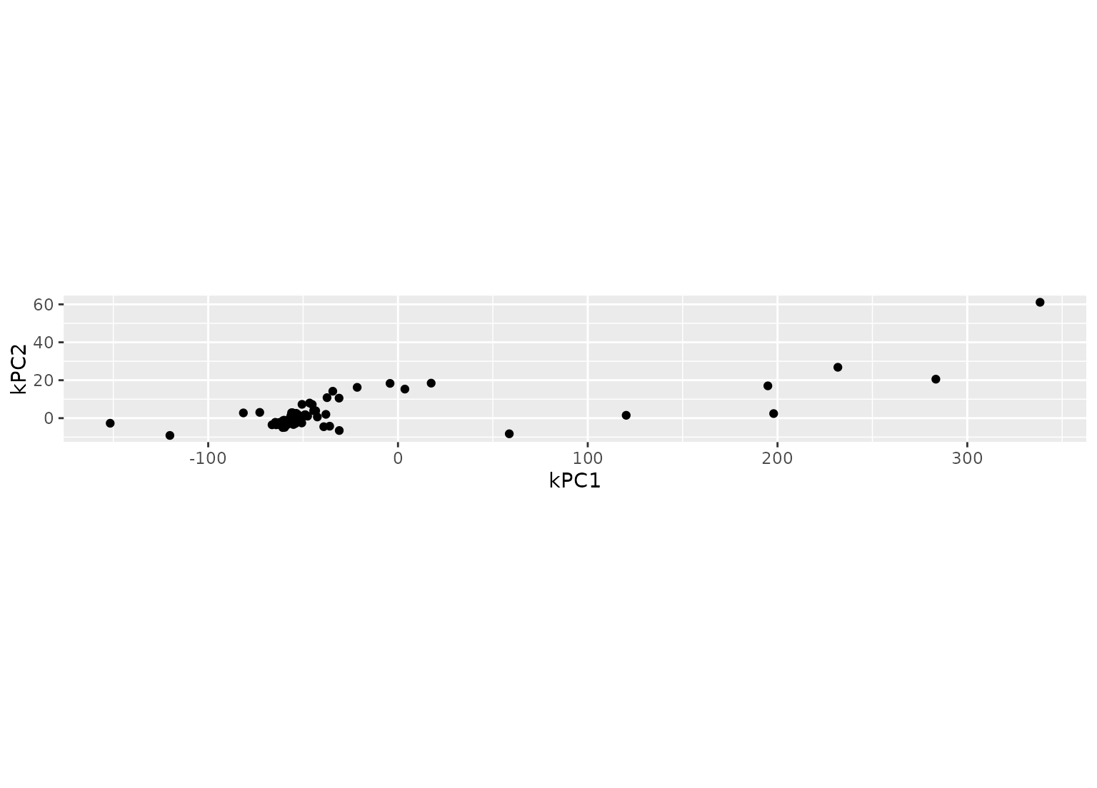
ggplot(kpca_te, aes(x = kPC1, y = kPC2)) +
  geom_point() +
  coord_equal()


tidy(kpca_trans, number = 3)
#> # A tibble: 1 × 2
#>   terms                    id             
#>   <chr>                    <chr>          
#> 1 all_numeric_predictors() kpca_poly_Qw9rI
tidy(kpca_estimates, number = 3)
#> # A tibble: 5 × 2
#>   terms    id             
#>   <chr>    <chr>          
#> 1 carbon   kpca_poly_Qw9rI
#> 2 hydrogen kpca_poly_Qw9rI
#> 3 oxygen   kpca_poly_Qw9rI
#> 4 nitrogen kpca_poly_Qw9rI
#> 5 sulfur   kpca_poly_Qw9rI