Analysis of Variance (Wald, LR, and F Statistics)
anova.rms.RdThe anova function automatically tests most meaningful hypotheses
in a design. For example, suppose that age and cholesterol are
predictors, and that a general interaction is modeled using a restricted
spline surface. anova prints Wald statistics (\(F\) statistics
for an ols fit) for testing linearity of age, linearity of
cholesterol, age effect (age + age by cholesterol interaction),
cholesterol effect (cholesterol + age by cholesterol interaction),
linearity of the age by cholesterol interaction (i.e., adequacy of the
simple age * cholesterol 1 d.f. product), linearity of the interaction
in age alone, and linearity of the interaction in cholesterol
alone. Joint tests of all interaction terms in the model and all
nonlinear terms in the model are also performed. For any multiple
d.f. effects for continuous variables that were not modeled through
rcs, pol, lsp, etc., tests of linearity will be
omitted. This applies to matrix predictors produced by e.g.
poly or ns.
For lrm, orm, cph, psm and Glm fits, the better likelihood
ratio chi-square tests may be obtained by specifying test='LR'.
Fits must use x=TRUE, y=TRUE to run LR tests. The tests are run
fairly efficiently by subsetting the design matrix rather than
recreating it.
print.anova.rms is the printing
method. plot.anova.rms draws dot charts depicting the importance
of variables in the model, as measured by Wald or LR \(\chi^2\),
\(\chi^2\) minus d.f., AIC, \(P\)-values, partial
\(R^2\), \(R^2\) for the whole model after deleting the effects in
question, or proportion of overall model \(R^2\) that is due to each
predictor. latex.anova.rms is the latex method. It
substitutes Greek/math symbols in column headings, uses boldface for
TOTAL lines, and constructs a caption. Then it passes the result
to latex.default for conversion to LaTeX.
When the anova table was converted to account for missing data
imputation by processMI, a separate function prmiInfo can
be used to print information related to imputation adjustments.
For Bayesian models such as blrm, anova computes relative
explained variation indexes (REV) based on approximate Wald statistics.
This uses the variance-covariance matrix of all of the posterior draws,
and the individual draws of betas, plus an overall summary from the
posterior mode/mean/median beta. Wald chi-squares assuming multivariate
normality of betas are computed just as with frequentist models, and for
each draw (or for the summary) the ratio of the partial Wald chi-square
to the total Wald statistic for the model is computed as REV.
The print method calls latex or html methods
depending on options(prType=). For
latex a table environment is not used and an ordinary
tabular is produced. When using html with Quarto or RMarkdown,
results='asis' need not be written in the chunk header.
html.anova.rms just calls latex.anova.rms.
# S3 method for class 'rms'
anova(object, ..., main.effect=FALSE, tol=.Machine$double.eps,
      test=c('F','Chisq','LR'), india=TRUE, indnl=TRUE, ss=TRUE,
      vnames=c('names','labels'),
      posterior.summary=c('mean', 'median', 'mode'), ns=500, cint=0.95,
      fitargs=NULL)

# S3 method for class 'anova.rms'
print(x,
      which=c('none','subscripts','names','dots'),
      table.env=FALSE, ...)

# S3 method for class 'anova.rms'
plot(x,
     what=c("chisqminusdf","chisq","aic","P","partial R2","remaining R2",
            "proportion R2", "proportion chisq"),
     xlab=NULL, pch=16,
     rm.totals=TRUE, rm.ia=FALSE, rm.other=NULL, newnames,
     sort=c("descending","ascending","none"), margin=c('chisq','P'),
     pl=TRUE, trans=NULL, ntrans=40, height=NULL, width=NULL, ...)

# S3 method for class 'anova.rms'
latex(object, title, dec.chisq=2,
      dec.F=2, dec.ss=NA, dec.ms=NA, dec.P=4, dec.REV=3,
      table.env=TRUE,
      caption=NULL, fontsize=1, params, ...)

# S3 method for class 'anova.rms'
html(object, ...)
Arguments
- object
a
rmsfit object.objectmust allowvcovto return the variance-covariance matrix. Forlatexis the result ofanova.- ...
If omitted, all variables are tested, yielding tests for individual factors and for pooled effects. Specify a subset of the variables to obtain tests for only those factors, with a pooled tests for the combined effects of all factors listed. Names may be abbreviated. For example, specify
anova(fit,age,cholesterol)to get a Wald statistic for testing the joint importance of age, cholesterol, and any factor interacting with them. Addtest='LR'to get a likelihood ratio chi-square test instead.Can be optional graphical parameters to send to
dotchart2, or other parameters to send tolatex.default. Ignored forprint.For
html.anova.rmsthe arguments are passed tolatex.anova.rms.- main.effect
Set to
TRUEto print the (usually meaningless) main effect tests even when the factor is involved in an interaction. The default isFALSE, to print only the effect of the main effect combined with all interactions involving that factor.- tol
singularity criterion for use in matrix inversion
- test
For an
olsfit, settest="Chisq"to use Wald \(\chi^2\) tests rather than F-tests. Forlrm, orm, cph, psmandGlmfits settest='LR'to get likelihood ratio \(\chi^2\) tests. This requires specifyingx=TRUE, y=TRUEwhen fitting the model.- india
set to
FALSEto exclude individual tests of interaction from the table- indnl
set to
FALSEto exclude individual tests of nonlinearity from the table- ss
For an
olsfit, setss=FALSEto suppress printing partial sums of squares, mean squares, and the Error SS and MS.- vnames
set to
'labels'to use variable labels rather than variable names in the output- posterior.summary
specifies whether the posterior mode/mean/median beta are to be used as a measure of central tendence of the posterior distribution, for use in relative explained variation from Bayesian models
- ns
number of random samples from the posterior draws to use for REV highest posterior density intervals
- cint
HPD interval probability
- fitargs
a list of extra arguments to be passed to the fitter for LR tests
- x
for
print,plot,textis the result ofanova.- which
If
whichis not"none"(the default),print.anova.rmswill add to the rightmost column of the output the list of parameters being tested by the hypothesis being tested in the current row. Specifyingwhich="subscripts"causes the subscripts of the regression coefficients being tested to be printed (with a subscript of one for the first non-intercept term).which="names"prints the names of the terms being tested, andwhich="dots"prints dots for terms being tested and blanks for those just being adjusted for.- what
what type of statistic to plot. The default is the \(\chi^2\) statistic for each factor (adding in the effect of higher-ordered factors containing that factor) minus its degrees of freedom. The R2 choices for
whatonly apply toolsmodels.- xlab
x-axis label, default is constructed according to
what.plotmathsymbols are used for R, by default.- pch
character for plotting dots in dot charts. Default is 16 (solid dot).
- rm.totals
set to
FALSEto keep total \(\chi^2\)s (overall, nonlinear, interaction totals) in the chart.- rm.ia
set to
TRUEto omit any effect that has"*"in its name- rm.other
a list of other predictor names to omit from the chart
- newnames
a list of substitute predictor names to use, after omitting any.
- sort
default is to sort bars in descending order of the summary statistic. Available options: 'ascending', 'descending', 'none'.
- margin
set to a vector of character strings to write text for selected statistics in the right margin of the dot chart. The character strings can be any combination of
"chisq","d.f.","P","partial R2","proportion R2", and"proportion chisq". Default is to not draw any statistics in the margin. Whenplotlyis in effect, margin values are instead displayed as hover text.- pl
set to
FALSEto suppress plotting. This is useful when you only wish to analyze the vector of statistics returned.- trans
set to a function to apply that transformation to the statistics being plotted, and to truncate negative values at zero. A good choice is
trans=sqrt.- ntrans
nargument topretty, specifying the number of values for which to place tick marks. This should be larger than usual because of nonlinear scaling, to provide a sufficient number of tick marks on the left (stretched) part of the chi-square scale.- height,width
height and width of
plotlyplots drawn usingdotchartp, in pixels. Ignored for ordinary plots. Defaults to minimum of 400 and 100 + 25 times the number of test statistics displayed.- title
title to pass to
latex, default is name of fit object passed toanovaprefixed with"anova.". For Windows, the default is"ano"followed by the first 5 letters of the name of the fit object.- dec.chisq
number of places to the right of the decimal place for typesetting \(\chi^2\) values (default is
2). Use zero for integer,NAfor floating point.- dec.F
digits to the right for \(F\) statistics (default is
2)- dec.ss
digits to the right for sums of squares (default is
NA, indicating floating point)- dec.ms
digits to the right for mean squares (default is
NA)- dec.P
digits to the right for \(P\)-values
- dec.REV
digits to the right for REV
- table.env
see
latex- caption
caption for table if
table.envisTRUE. Default is constructed from the response variable.- fontsize
font size for html output; default is 1 for
1em- params
used internally when called through print.
Value
anova.rms returns a matrix of class anova.rms containing factors
as rows and \(\chi^2\), d.f., and \(P\)-values as
columns (or d.f., partial \(SS, MS, F, P\)). An attribute
vinfo provides list of variables involved in each row and the
type of test done.
plot.anova.rms invisibly returns the vector of quantities
plotted. This vector has a names attribute describing the terms for
which the statistics in the vector are calculated.
Details
If the statistics being plotted with plot.anova.rms are few in
number and one of them is negative or zero, plot.anova.rms
will quit because of an error in dotchart2.
The latex method requires LaTeX packages relsize and
needspace.
Side Effects
print prints, latex creates a
file with a name of the form "title.tex" (see the title argument above).
See also
Examples
require(ggplot2)
#> Loading required package: ggplot2
n <- 1000 # define sample size
set.seed(17) # so can reproduce the results
treat <- factor(sample(c('a','b','c'), n,TRUE))
num.diseases <- sample(0:4, n,TRUE)
age <- rnorm(n, 50, 10)
cholesterol <- rnorm(n, 200, 25)
weight <- rnorm(n, 150, 20)
sex <- factor(sample(c('female','male'), n,TRUE))
label(age) <- 'Age' # label is in Hmisc
label(num.diseases) <- 'Number of Comorbid Diseases'
label(cholesterol) <- 'Total Cholesterol'
label(weight) <- 'Weight, lbs.'
label(sex) <- 'Sex'
units(cholesterol) <- 'mg/dl' # uses units.default in Hmisc
# Specify population model for log odds that Y=1
L <- .1*(num.diseases-2) + .045*(age-50) +
(log(cholesterol - 10)-5.2)*(-2*(treat=='a') +
3.5*(treat=='b')+2*(treat=='c'))
# Simulate binary y to have Prob(y=1) = 1/[1+exp(-L)]
y <- ifelse(runif(n) < plogis(L), 1, 0)
fit <- lrm(y ~ treat + scored(num.diseases) + rcs(age) +
log(cholesterol+10) + treat:log(cholesterol+10),
x=TRUE, y=TRUE) # x, y needed for test='LR'
#> number of knots in rcs defaulting to 5
a <- anova(fit) # Test all factors
b <- anova(fit, treat, cholesterol) # Test these 2 by themselves
# to get their pooled effects
a
#> Wald Statistics Response: y
#>
#> Factor Chi-Square d.f. P
#> treat (Factor+Higher Order Factors) 15.88 4 0.0032
#> All Interactions 10.79 2 0.0045
#> num.diseases 14.91 4 0.0049
#> Nonlinear 0.73 3 0.8660
#> age 67.97 4 <.0001
#> Nonlinear 1.11 3 0.7738
#> cholesterol (Factor+Higher Order Factors) 12.99 3 0.0047
#> All Interactions 10.79 2 0.0045
#> treat * cholesterol (Factor+Higher Order Factors) 10.79 2 0.0045
#> TOTAL NONLINEAR 2.03 6 0.9168
#> TOTAL NONLINEAR + INTERACTION 13.20 8 0.1051
#> TOTAL 90.80 13 <.0001
b
#> Wald Statistics Response: y
#>
#> Factor Chi-Square d.f. P
#> treat (Factor+Higher Order Factors) 15.88 4 0.0032
#> All Interactions 10.79 2 0.0045
#> cholesterol (Factor+Higher Order Factors) 12.99 3 0.0047
#> All Interactions 10.79 2 0.0045
#> TOTAL 17.90 5 0.0031
a2 <- anova(fit, test='LR')
b2 <- anova(fit, treat, cholesterol, test='LR')
a2
#> Likelihood Ratio Statistics Response: y
#>
#> Factor Chi-Square d.f. P
#> treat (Factor+Higher Order Factors) 16.29 4 0.0027
#> All Interactions 11.01 2 0.0041
#> num.diseases 15.09 4 0.0045
#> Nonlinear 0.73 3 0.8657
#> age 75.40 4 <.0001
#> Nonlinear 1.11 3 0.7739
#> cholesterol (Factor+Higher Order Factors) 13.38 3 0.0039
#> All Interactions 11.01 2 0.0041
#> treat * cholesterol (Factor+Higher Order Factors) 11.01 2 0.0041
#> TOTAL NONLINEAR 2.03 6 0.9165
#> TOTAL NONLINEAR + INTERACTION 13.55 8 0.0943
#> TOTAL 105.73 13 <.0001
b2
#> Likelihood Ratio Statistics Response: y
#>
#> Factor Chi-Square d.f. P
#> treat (Factor+Higher Order Factors) 16.29 4 0.0027
#> All Interactions 11.01 2 0.0041
#> cholesterol (Factor+Higher Order Factors) 13.38 3 0.0039
#> All Interactions 11.01 2 0.0041
#> TOTAL 18.56 5 0.0023
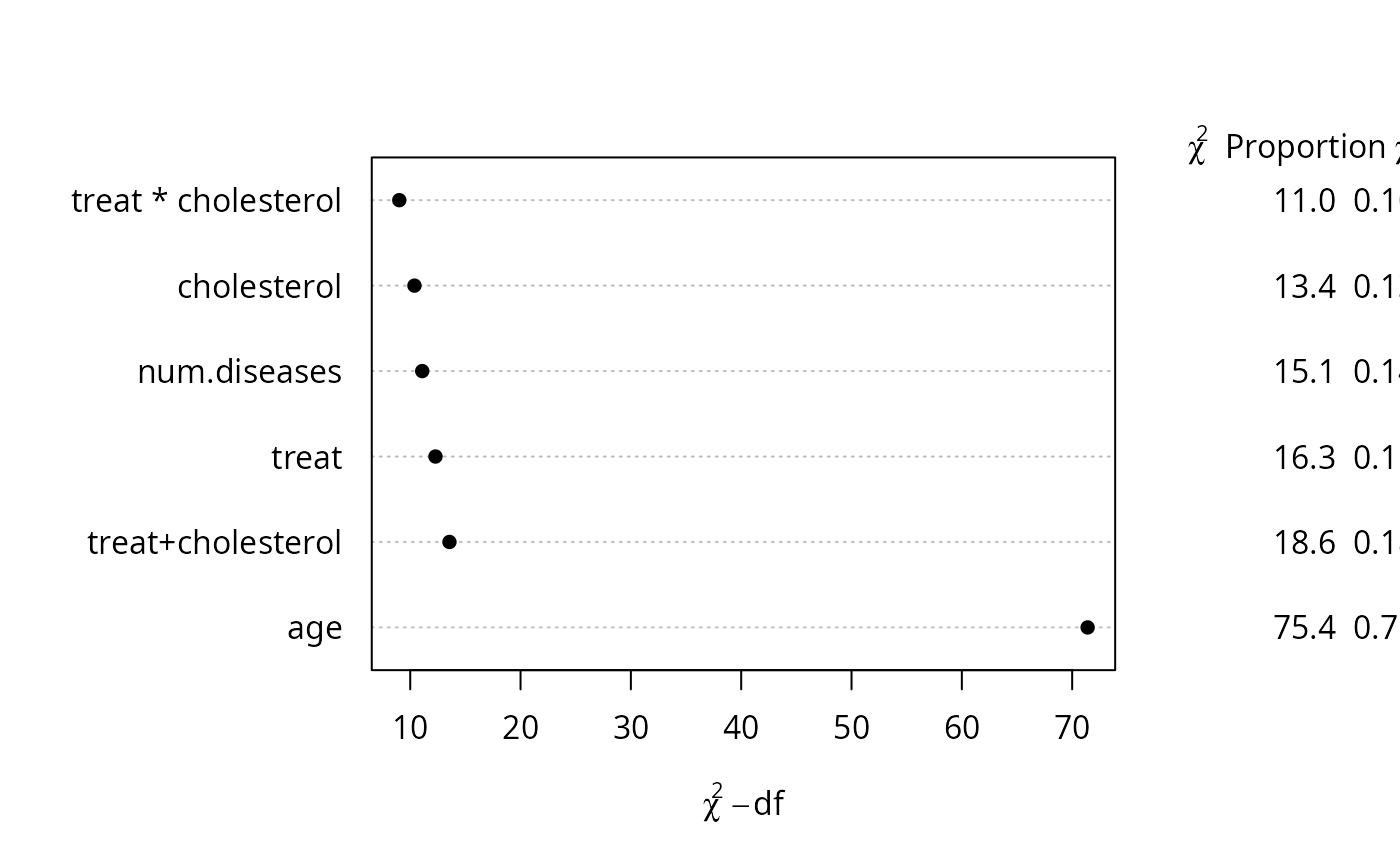
# Add a new line to the plot with combined effects
s <- rbind(a2, 'treat+cholesterol'=b2['TOTAL',])
class(s) <- 'anova.rms'
plot(s, margin=c('chisq', 'proportion chisq'))
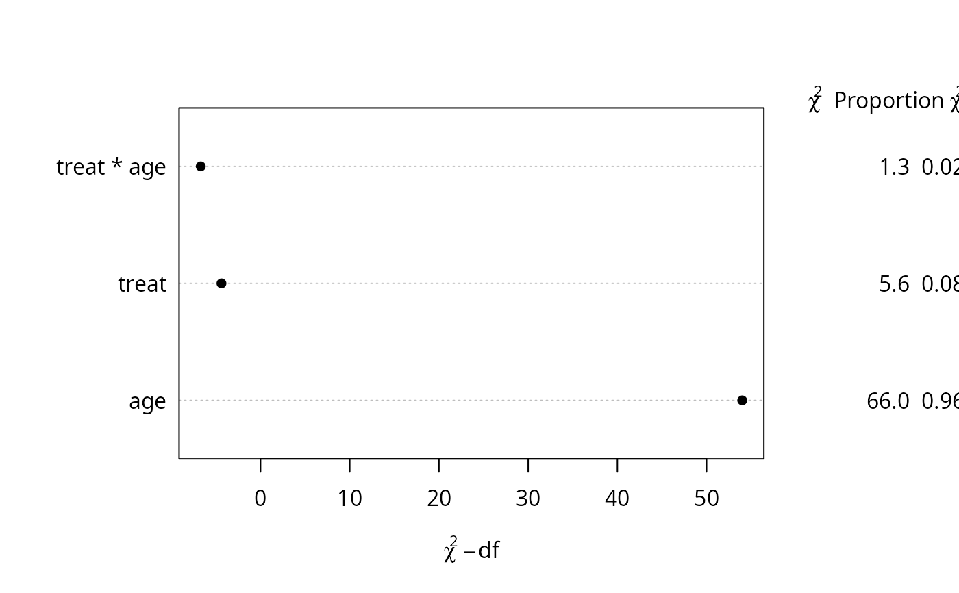
 g <- lrm(y ~ treat*rcs(age))
#> number of knots in rcs defaulting to 5
dd <- datadist(treat, num.diseases, age, cholesterol)
options(datadist='dd')
p <- Predict(g, age, treat="b")
#> Error in value.chk(at, which(name == n), NA, np, lim): variable age does not have limits defined by datadist
s <- anova(g)
tx <- paste(capture.output(s), collapse='\n')
ggplot(p) + annotate('text', x=27, y=3.2, family='mono', label=tx,
hjust=0, vjust=1, size=1.5)
#> Error: object 'p' not found
plot(s, margin=c('chisq', 'proportion chisq'))
g <- lrm(y ~ treat*rcs(age))
#> number of knots in rcs defaulting to 5
dd <- datadist(treat, num.diseases, age, cholesterol)
options(datadist='dd')
p <- Predict(g, age, treat="b")
#> Error in value.chk(at, which(name == n), NA, np, lim): variable age does not have limits defined by datadist
s <- anova(g)
tx <- paste(capture.output(s), collapse='\n')
ggplot(p) + annotate('text', x=27, y=3.2, family='mono', label=tx,
hjust=0, vjust=1, size=1.5)
#> Error: object 'p' not found
plot(s, margin=c('chisq', 'proportion chisq'))
 # new plot - dot chart of chisq-d.f. with 2 other stats in right margin
# latex(s) # nice printout - creates anova.g.tex
options(datadist=NULL)
# Simulate data with from a given model, and display exactly which
# hypotheses are being tested
set.seed(123)
age <- rnorm(500, 50, 15)
treat <- factor(sample(c('a','b','c'), 500, TRUE))
bp <- rnorm(500, 120, 10)
y <- ifelse(treat=='a', (age-50)*.05, abs(age-50)*.08) + 3*(treat=='c') +
pmax(bp, 100)*.09 + rnorm(500)
f <- ols(y ~ treat*lsp(age,50) + rcs(bp,4))
print(names(coef(f)), quote=FALSE)
#> [1] Intercept treat=b treat=c age age'
#> [6] bp bp' bp'' treat=b * age treat=c * age
#> [11] treat=b * age' treat=c * age'
specs(f)
#> ols(formula = y ~ treat * lsp(age, 50) + rcs(bp, 4))
#>
#> Assumption Parameters d.f.
#> treat category a b c 2
#> age lspline 50 2
#> bp rcspline 103.28 116.6 123.63 137.53 3
#> treat * age interaction linear x nonlinear - Ag(B) 4
anova(f)
#> Analysis of Variance Response: y
#>
#> Factor d.f. Partial SS MS F
#> treat (Factor+Higher Order Factors) 6 1421.697707 236.9496179 241.73
#> All Interactions 4 61.546142 15.3865356 15.70
#> age (Factor+Higher Order Factors) 6 222.006522 37.0010869 37.75
#> All Interactions 4 61.546142 15.3865356 15.70
#> Nonlinear (Factor+Higher Order Factors) 3 156.880935 52.2936449 53.35
#> bp 3 344.332965 114.7776551 117.09
#> Nonlinear 2 1.411244 0.7056222 0.72
#> treat * age (Factor+Higher Order Factors) 4 61.546142 15.3865356 15.70
#> Nonlinear 2 22.872076 11.4360378 11.67
#> Nonlinear Interaction : f(A,B) vs. AB 2 22.872076 11.4360378 11.67
#> TOTAL NONLINEAR 5 157.749868 31.5499735 32.19
#> TOTAL NONLINEAR + INTERACTION 7 194.532234 27.7903192 28.35
#> REGRESSION 11 1861.112468 169.1920425 172.61
#> ERROR 488 478.347327 0.9802199
#> P
#> <.0001
#> <.0001
#> <.0001
#> <.0001
#> <.0001
#> <.0001
#> 0.4873
#> <.0001
#> <.0001
#> <.0001
#> <.0001
#> <.0001
#> <.0001
#>
an <- anova(f)
options(digits=3)
print(an, 'subscripts')
#> Analysis of Variance Response: y
#>
#> Factor d.f. Partial SS MS F
#> treat (Factor+Higher Order Factors) 6 1421.70 236.950 241.73
#> All Interactions 4 61.55 15.387 15.70
#> age (Factor+Higher Order Factors) 6 222.01 37.001 37.75
#> All Interactions 4 61.55 15.387 15.70
#> Nonlinear (Factor+Higher Order Factors) 3 156.88 52.294 53.35
#> bp 3 344.33 114.778 117.09
#> Nonlinear 2 1.41 0.706 0.72
#> treat * age (Factor+Higher Order Factors) 4 61.55 15.387 15.70
#> Nonlinear 2 22.87 11.436 11.67
#> Nonlinear Interaction : f(A,B) vs. AB 2 22.87 11.436 11.67
#> TOTAL NONLINEAR 5 157.75 31.550 32.19
#> TOTAL NONLINEAR + INTERACTION 7 194.53 27.790 28.35
#> REGRESSION 11 1861.11 169.192 172.61
#> ERROR 488 478.35 0.980
#> P Tested
#> <.0001 1-2,8-11
#> <.0001 8-11
#> <.0001 3-4,8-11
#> <.0001 8-11
#> <.0001 4,10-11
#> <.0001 5-7
#> 0.487 6-7
#> <.0001 8-11
#> <.0001 10-11
#> <.0001 10-11
#> <.0001 4,6-7,10-11
#> <.0001 4,6-11
#> <.0001 1-11
#>
#>
#> Subscripts correspond to:
#> [1] treat=b treat=c age age' bp
#> [6] bp' bp'' treat=b * age treat=c * age treat=b * age'
#> [11] treat=c * age'
print(an, 'dots')
#> Analysis of Variance Response: y
#>
#> Factor d.f. Partial SS MS F
#> treat (Factor+Higher Order Factors) 6 1421.70 236.950 241.73
#> All Interactions 4 61.55 15.387 15.70
#> age (Factor+Higher Order Factors) 6 222.01 37.001 37.75
#> All Interactions 4 61.55 15.387 15.70
#> Nonlinear (Factor+Higher Order Factors) 3 156.88 52.294 53.35
#> bp 3 344.33 114.778 117.09
#> Nonlinear 2 1.41 0.706 0.72
#> treat * age (Factor+Higher Order Factors) 4 61.55 15.387 15.70
#> Nonlinear 2 22.87 11.436 11.67
#> Nonlinear Interaction : f(A,B) vs. AB 2 22.87 11.436 11.67
#> TOTAL NONLINEAR 5 157.75 31.550 32.19
#> TOTAL NONLINEAR + INTERACTION 7 194.53 27.790 28.35
#> REGRESSION 11 1861.11 169.192 172.61
#> ERROR 488 478.35 0.980
#> P Tested
#> <.0001 .. ....
#> <.0001 ....
#> <.0001 .. ....
#> <.0001 ....
#> <.0001 . ..
#> <.0001 ...
#> 0.487 ..
#> <.0001 ....
#> <.0001 ..
#> <.0001 ..
#> <.0001 . .. ..
#> <.0001 . ......
#> <.0001 ...........
#>
#>
#> Subscripts correspond to:
#> [1] treat=b treat=c age age' bp
#> [6] bp' bp'' treat=b * age treat=c * age treat=b * age'
#> [11] treat=c * age'
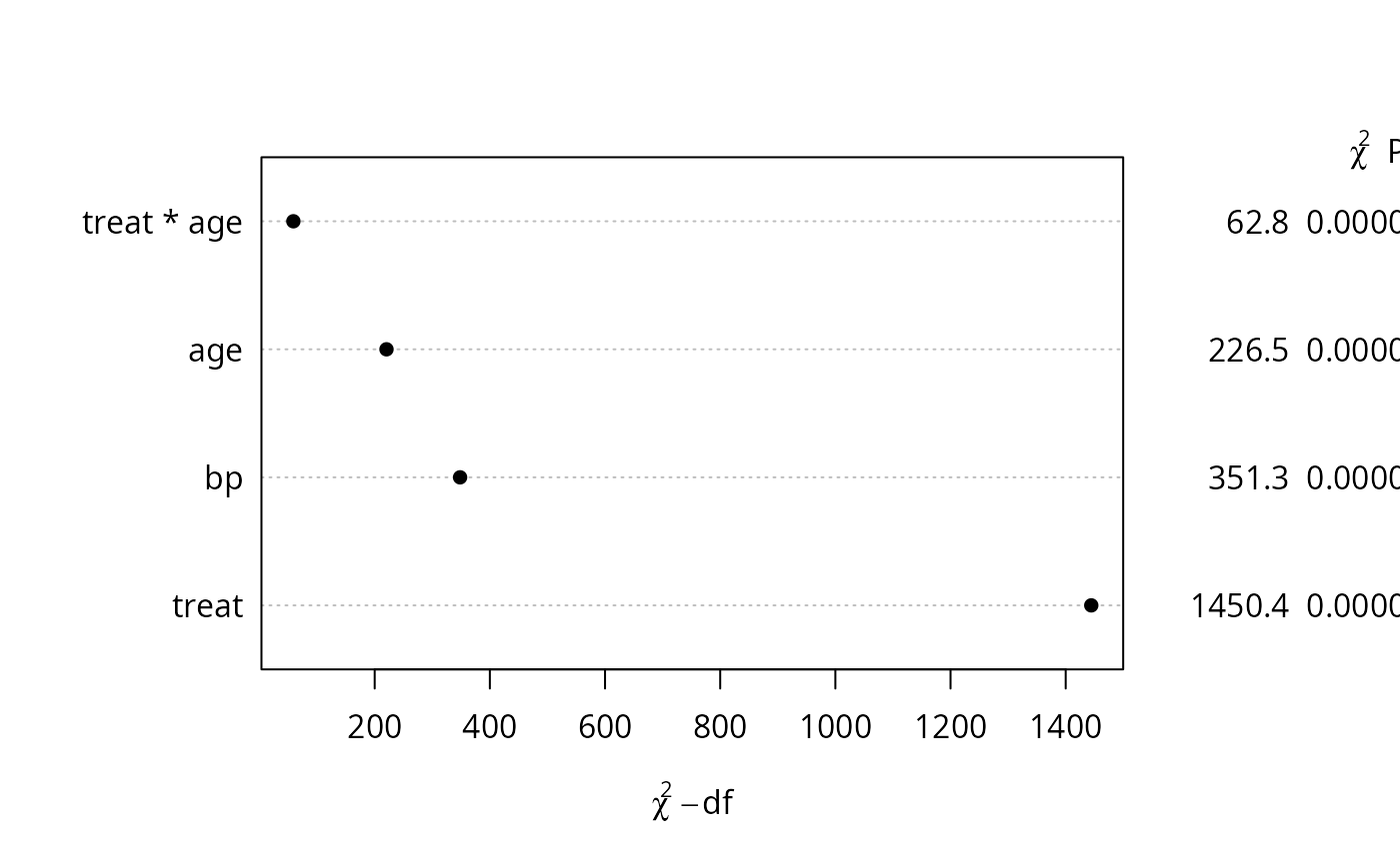
an <- anova(f, test='Chisq', ss=FALSE)
# plot(0:1) # make some plot
# tab <- pantext(an, 1.2, .6, lattice=FALSE, fontfamily='Helvetica')
# create function to write table; usually omit fontfamily
# tab() # execute it; could do tab(cex=.65)
plot(an) # new plot - dot chart of chisq-d.f.
# new plot - dot chart of chisq-d.f. with 2 other stats in right margin
# latex(s) # nice printout - creates anova.g.tex
options(datadist=NULL)
# Simulate data with from a given model, and display exactly which
# hypotheses are being tested
set.seed(123)
age <- rnorm(500, 50, 15)
treat <- factor(sample(c('a','b','c'), 500, TRUE))
bp <- rnorm(500, 120, 10)
y <- ifelse(treat=='a', (age-50)*.05, abs(age-50)*.08) + 3*(treat=='c') +
pmax(bp, 100)*.09 + rnorm(500)
f <- ols(y ~ treat*lsp(age,50) + rcs(bp,4))
print(names(coef(f)), quote=FALSE)
#> [1] Intercept treat=b treat=c age age'
#> [6] bp bp' bp'' treat=b * age treat=c * age
#> [11] treat=b * age' treat=c * age'
specs(f)
#> ols(formula = y ~ treat * lsp(age, 50) + rcs(bp, 4))
#>
#> Assumption Parameters d.f.
#> treat category a b c 2
#> age lspline 50 2
#> bp rcspline 103.28 116.6 123.63 137.53 3
#> treat * age interaction linear x nonlinear - Ag(B) 4
anova(f)
#> Analysis of Variance Response: y
#>
#> Factor d.f. Partial SS MS F
#> treat (Factor+Higher Order Factors) 6 1421.697707 236.9496179 241.73
#> All Interactions 4 61.546142 15.3865356 15.70
#> age (Factor+Higher Order Factors) 6 222.006522 37.0010869 37.75
#> All Interactions 4 61.546142 15.3865356 15.70
#> Nonlinear (Factor+Higher Order Factors) 3 156.880935 52.2936449 53.35
#> bp 3 344.332965 114.7776551 117.09
#> Nonlinear 2 1.411244 0.7056222 0.72
#> treat * age (Factor+Higher Order Factors) 4 61.546142 15.3865356 15.70
#> Nonlinear 2 22.872076 11.4360378 11.67
#> Nonlinear Interaction : f(A,B) vs. AB 2 22.872076 11.4360378 11.67
#> TOTAL NONLINEAR 5 157.749868 31.5499735 32.19
#> TOTAL NONLINEAR + INTERACTION 7 194.532234 27.7903192 28.35
#> REGRESSION 11 1861.112468 169.1920425 172.61
#> ERROR 488 478.347327 0.9802199
#> P
#> <.0001
#> <.0001
#> <.0001
#> <.0001
#> <.0001
#> <.0001
#> 0.4873
#> <.0001
#> <.0001
#> <.0001
#> <.0001
#> <.0001
#> <.0001
#>
an <- anova(f)
options(digits=3)
print(an, 'subscripts')
#> Analysis of Variance Response: y
#>
#> Factor d.f. Partial SS MS F
#> treat (Factor+Higher Order Factors) 6 1421.70 236.950 241.73
#> All Interactions 4 61.55 15.387 15.70
#> age (Factor+Higher Order Factors) 6 222.01 37.001 37.75
#> All Interactions 4 61.55 15.387 15.70
#> Nonlinear (Factor+Higher Order Factors) 3 156.88 52.294 53.35
#> bp 3 344.33 114.778 117.09
#> Nonlinear 2 1.41 0.706 0.72
#> treat * age (Factor+Higher Order Factors) 4 61.55 15.387 15.70
#> Nonlinear 2 22.87 11.436 11.67
#> Nonlinear Interaction : f(A,B) vs. AB 2 22.87 11.436 11.67
#> TOTAL NONLINEAR 5 157.75 31.550 32.19
#> TOTAL NONLINEAR + INTERACTION 7 194.53 27.790 28.35
#> REGRESSION 11 1861.11 169.192 172.61
#> ERROR 488 478.35 0.980
#> P Tested
#> <.0001 1-2,8-11
#> <.0001 8-11
#> <.0001 3-4,8-11
#> <.0001 8-11
#> <.0001 4,10-11
#> <.0001 5-7
#> 0.487 6-7
#> <.0001 8-11
#> <.0001 10-11
#> <.0001 10-11
#> <.0001 4,6-7,10-11
#> <.0001 4,6-11
#> <.0001 1-11
#>
#>
#> Subscripts correspond to:
#> [1] treat=b treat=c age age' bp
#> [6] bp' bp'' treat=b * age treat=c * age treat=b * age'
#> [11] treat=c * age'
print(an, 'dots')
#> Analysis of Variance Response: y
#>
#> Factor d.f. Partial SS MS F
#> treat (Factor+Higher Order Factors) 6 1421.70 236.950 241.73
#> All Interactions 4 61.55 15.387 15.70
#> age (Factor+Higher Order Factors) 6 222.01 37.001 37.75
#> All Interactions 4 61.55 15.387 15.70
#> Nonlinear (Factor+Higher Order Factors) 3 156.88 52.294 53.35
#> bp 3 344.33 114.778 117.09
#> Nonlinear 2 1.41 0.706 0.72
#> treat * age (Factor+Higher Order Factors) 4 61.55 15.387 15.70
#> Nonlinear 2 22.87 11.436 11.67
#> Nonlinear Interaction : f(A,B) vs. AB 2 22.87 11.436 11.67
#> TOTAL NONLINEAR 5 157.75 31.550 32.19
#> TOTAL NONLINEAR + INTERACTION 7 194.53 27.790 28.35
#> REGRESSION 11 1861.11 169.192 172.61
#> ERROR 488 478.35 0.980
#> P Tested
#> <.0001 .. ....
#> <.0001 ....
#> <.0001 .. ....
#> <.0001 ....
#> <.0001 . ..
#> <.0001 ...
#> 0.487 ..
#> <.0001 ....
#> <.0001 ..
#> <.0001 ..
#> <.0001 . .. ..
#> <.0001 . ......
#> <.0001 ...........
#>
#>
#> Subscripts correspond to:
#> [1] treat=b treat=c age age' bp
#> [6] bp' bp'' treat=b * age treat=c * age treat=b * age'
#> [11] treat=c * age'
an <- anova(f, test='Chisq', ss=FALSE)
# plot(0:1) # make some plot
# tab <- pantext(an, 1.2, .6, lattice=FALSE, fontfamily='Helvetica')
# create function to write table; usually omit fontfamily
# tab() # execute it; could do tab(cex=.65)
plot(an) # new plot - dot chart of chisq-d.f.
 # Specify plot(an, trans=sqrt) to use a square root scale for this plot
# latex(an) # nice printout - creates anova.f.tex
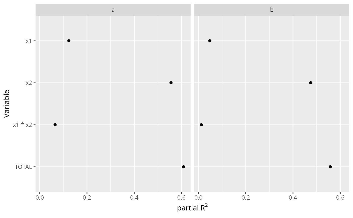
## Example to save partial R^2 for all predictors, along with overall
## R^2, from two separate fits, and to combine them with ggplot2
require(ggplot2)
set.seed(1)
n <- 100
x1 <- runif(n)
x2 <- runif(n)
y <- (x1-.5)^2 + x2 + runif(n)
group <- c(rep('a', n/2), rep('b', n/2))
A <- NULL
for(g in c('a','b')) {
f <- ols(y ~ pol(x1,2) + pol(x2,2) + pol(x1,2) %ia% pol(x2,2),
subset=group==g)
a <- plot(anova(f),
what='partial R2', pl=FALSE, rm.totals=FALSE, sort='none')
a <- a[-grep('NONLINEAR', names(a))]
d <- data.frame(group=g, Variable=factor(names(a), names(a)),
partialR2=unname(a))
A <- rbind(A, d)
}
ggplot(A, aes(x=partialR2, y=Variable)) + geom_point() +
facet_wrap(~ group) + xlab(ex <- expression(partial~R^2)) +
scale_y_discrete(limits=rev)
# Specify plot(an, trans=sqrt) to use a square root scale for this plot
# latex(an) # nice printout - creates anova.f.tex
## Example to save partial R^2 for all predictors, along with overall
## R^2, from two separate fits, and to combine them with ggplot2
require(ggplot2)
set.seed(1)
n <- 100
x1 <- runif(n)
x2 <- runif(n)
y <- (x1-.5)^2 + x2 + runif(n)
group <- c(rep('a', n/2), rep('b', n/2))
A <- NULL
for(g in c('a','b')) {
f <- ols(y ~ pol(x1,2) + pol(x2,2) + pol(x1,2) %ia% pol(x2,2),
subset=group==g)
a <- plot(anova(f),
what='partial R2', pl=FALSE, rm.totals=FALSE, sort='none')
a <- a[-grep('NONLINEAR', names(a))]
d <- data.frame(group=g, Variable=factor(names(a), names(a)),
partialR2=unname(a))
A <- rbind(A, d)
}
ggplot(A, aes(x=partialR2, y=Variable)) + geom_point() +
facet_wrap(~ group) + xlab(ex <- expression(partial~R^2)) +
scale_y_discrete(limits=rev)
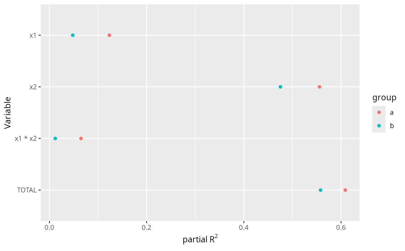
 ggplot(A, aes(x=partialR2, y=Variable, color=group)) + geom_point() +
xlab(ex <- expression(partial~R^2)) +
scale_y_discrete(limits=rev)
ggplot(A, aes(x=partialR2, y=Variable, color=group)) + geom_point() +
xlab(ex <- expression(partial~R^2)) +
scale_y_discrete(limits=rev)
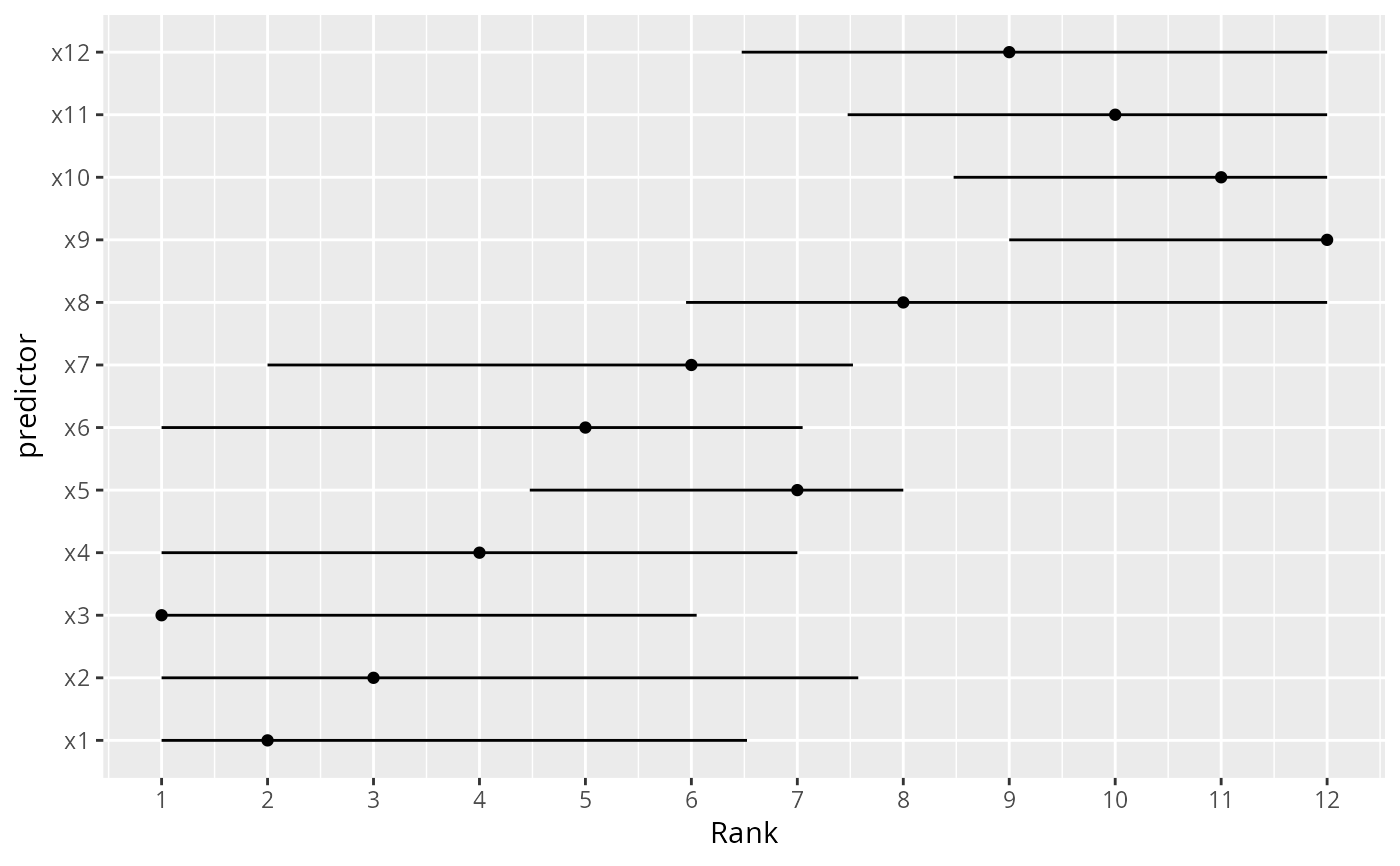
 # Suppose that a researcher wants to make a big deal about a variable
# because it has the highest adjusted chi-square. We use the
# bootstrap to derive 0.95 confidence intervals for the ranks of all
# the effects in the model. We use the plot method for anova, with
# pl=FALSE to suppress actual plotting of chi-square - d.f. for each
# bootstrap repetition.
# It is important to tell plot.anova.rms not to sort the results, or
# every bootstrap replication would have ranks of 1,2,3,... for the stats.
n <- 300
set.seed(1)
d <- data.frame(x1=runif(n), x2=runif(n), x3=runif(n),
x4=runif(n), x5=runif(n), x6=runif(n), x7=runif(n),
x8=runif(n), x9=runif(n), x10=runif(n), x11=runif(n),
x12=runif(n))
d$y <- with(d, 1*x1 + 2*x2 + 3*x3 + 4*x4 + 5*x5 + 6*x6 +
7*x7 + 8*x8 + 9*x9 + 10*x10 + 11*x11 +
12*x12 + 9*rnorm(n))
f <- ols(y ~ x1+x2+x3+x4+x5+x6+x7+x8+x9+x10+x11+x12, data=d)
B <- 20 # actually use B=1000
ranks <- matrix(NA, nrow=B, ncol=12)
rankvars <- function(fit)
rank(plot(anova(fit), sort='none', pl=FALSE))
Rank <- rankvars(f)
for(i in 1:B) {
j <- sample(1:n, n, TRUE)
bootfit <- update(f, data=d, subset=j)
ranks[i,] <- rankvars(bootfit)
}
lim <- t(apply(ranks, 2, quantile, probs=c(.025,.975)))
predictor <- factor(names(Rank), names(Rank))
w <- data.frame(predictor, Rank, lower=lim[,1], upper=lim[,2])
ggplot(w, aes(x=predictor, y=Rank)) + geom_point() + coord_flip() +
scale_y_continuous(breaks=1:12) +
geom_errorbar(aes(ymin=lim[,1], ymax=lim[,2]), width=0)
# Suppose that a researcher wants to make a big deal about a variable
# because it has the highest adjusted chi-square. We use the
# bootstrap to derive 0.95 confidence intervals for the ranks of all
# the effects in the model. We use the plot method for anova, with
# pl=FALSE to suppress actual plotting of chi-square - d.f. for each
# bootstrap repetition.
# It is important to tell plot.anova.rms not to sort the results, or
# every bootstrap replication would have ranks of 1,2,3,... for the stats.
n <- 300
set.seed(1)
d <- data.frame(x1=runif(n), x2=runif(n), x3=runif(n),
x4=runif(n), x5=runif(n), x6=runif(n), x7=runif(n),
x8=runif(n), x9=runif(n), x10=runif(n), x11=runif(n),
x12=runif(n))
d$y <- with(d, 1*x1 + 2*x2 + 3*x3 + 4*x4 + 5*x5 + 6*x6 +
7*x7 + 8*x8 + 9*x9 + 10*x10 + 11*x11 +
12*x12 + 9*rnorm(n))
f <- ols(y ~ x1+x2+x3+x4+x5+x6+x7+x8+x9+x10+x11+x12, data=d)
B <- 20 # actually use B=1000
ranks <- matrix(NA, nrow=B, ncol=12)
rankvars <- function(fit)
rank(plot(anova(fit), sort='none', pl=FALSE))
Rank <- rankvars(f)
for(i in 1:B) {
j <- sample(1:n, n, TRUE)
bootfit <- update(f, data=d, subset=j)
ranks[i,] <- rankvars(bootfit)
}
lim <- t(apply(ranks, 2, quantile, probs=c(.025,.975)))
predictor <- factor(names(Rank), names(Rank))
w <- data.frame(predictor, Rank, lower=lim[,1], upper=lim[,2])
ggplot(w, aes(x=predictor, y=Rank)) + geom_point() + coord_flip() +
scale_y_continuous(breaks=1:12) +
geom_errorbar(aes(ymin=lim[,1], ymax=lim[,2]), width=0)