Nonparametric Survival Estimates for Censored Data
npsurv.RdComputes an estimate of a survival curve for censored data
using either the Kaplan-Meier or the Fleming-Harrington method
or computes the predicted survivor function.
For competing risks data it computes the cumulative incidence curve.
This calls the survival package's survfit.formula
function. Attributes of the event time variable are saved (label and
units of measurement).
For competing risks the second argument for Surv should be the
event state variable, and it should be a factor variable with the first
factor level denoting right-censored observations.
npsurv(formula, data=environment(formula),
              subset, weights, na.action=na.delete, ...)
Arguments
- formula
a formula object, which must have a
Survobject as the response on the left of the~operator and, if desired, terms separated by + operators on the right. One of the terms may be astrataobject. For a single survival curve the right hand side should be~ 1.- data,subset,weights,na.action
see
survfit.formula- ...
see
survfit.formula
Value
an object of class "npsurv" and "survfit".
See survfit.object for details. Methods defined for survfit
objects are print, summary, plot,lines, and
points.
Details
see survfit.formula for details
See also
survfit.cph for survival curves from Cox models.
print,
plot,
lines,
coxph,
strata,
survplot, ggplot.npsurv
Examples
require(survival)
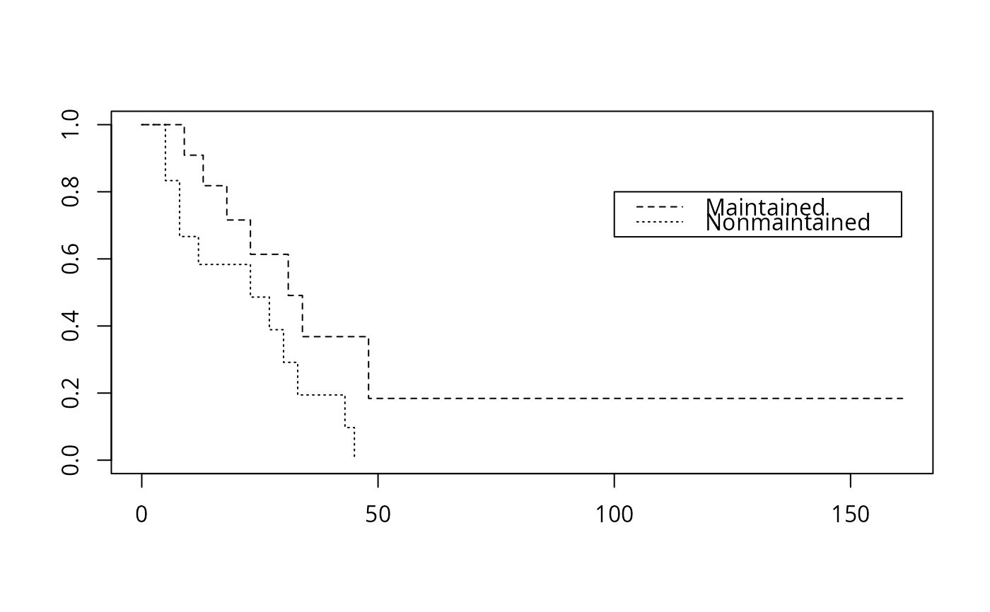
# fit a Kaplan-Meier and plot it
fit <- npsurv(Surv(time, status) ~ x, data = aml)
plot(fit, lty = 2:3)
legend(100, .8, c("Maintained", "Nonmaintained"), lty = 2:3)
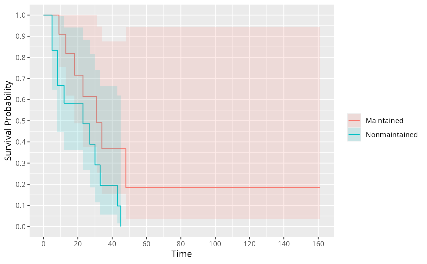
 ggplot(fit) # prettier than plot()
 # Here is the data set from Turnbull
# There are no interval censored subjects, only left-censored (status=3),
# right-censored (status 0) and observed events (status 1)
#
# Time
# 1 2 3 4
# Type of observation
# death 12 6 2 3
# losses 3 2 0 3
# late entry 2 4 2 5
#
tdata <- data.frame(time = c(1,1,1,2,2,2,3,3,3,4,4,4),
status = rep(c(1,0,2),4),
n = c(12,3,2,6,2,4,2,0,2,3,3,5))
fit <- npsurv(Surv(time, time, status, type='interval') ~ 1,
data=tdata, weights=n)
#
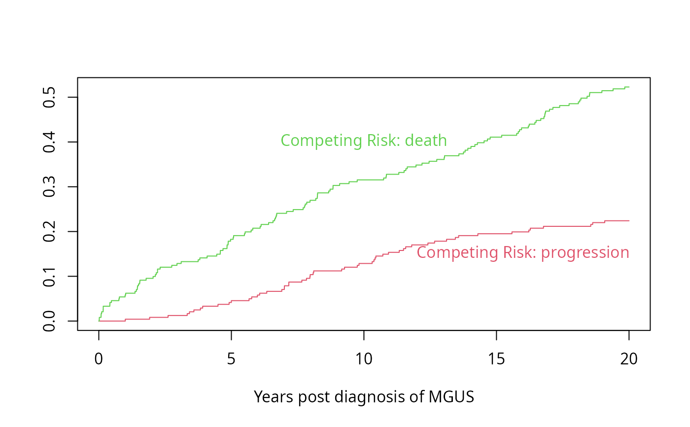
# Time to progression/death for patients with monoclonal gammopathy
# Competing risk curves (cumulative incidence)
# status variable must be a factor with first level denoting right censoring
m <- upData(mgus1, stop = stop / 365.25, units=c(stop='years'),
labels=c(stop='Follow-up Time'), subset=start == 0)
#> Input object size: 35552 bytes; 14 variables 305 observations
#> Modified variable stop
#> New object size: 25104 bytes; 14 variables 241 observations
f <- npsurv(Surv(stop, event) ~ 1, data=m)
# CI curves are always plotted from 0 upwards, rather than 1 down
plot(f, fun='event', xmax=20, mark.time=FALSE,
col=2:3, xlab="Years post diagnosis of MGUS")
text(10, .4, "Competing Risk: death", col=3)
text(16, .15,"Competing Risk: progression", col=2)
# Here is the data set from Turnbull
# There are no interval censored subjects, only left-censored (status=3),
# right-censored (status 0) and observed events (status 1)
#
# Time
# 1 2 3 4
# Type of observation
# death 12 6 2 3
# losses 3 2 0 3
# late entry 2 4 2 5
#
tdata <- data.frame(time = c(1,1,1,2,2,2,3,3,3,4,4,4),
status = rep(c(1,0,2),4),
n = c(12,3,2,6,2,4,2,0,2,3,3,5))
fit <- npsurv(Surv(time, time, status, type='interval') ~ 1,
data=tdata, weights=n)
#
# Time to progression/death for patients with monoclonal gammopathy
# Competing risk curves (cumulative incidence)
# status variable must be a factor with first level denoting right censoring
m <- upData(mgus1, stop = stop / 365.25, units=c(stop='years'),
labels=c(stop='Follow-up Time'), subset=start == 0)
#> Input object size: 35552 bytes; 14 variables 305 observations
#> Modified variable stop
#> New object size: 25104 bytes; 14 variables 241 observations
f <- npsurv(Surv(stop, event) ~ 1, data=m)
# CI curves are always plotted from 0 upwards, rather than 1 down
plot(f, fun='event', xmax=20, mark.time=FALSE,
col=2:3, xlab="Years post diagnosis of MGUS")
text(10, .4, "Competing Risk: death", col=3)
text(16, .15,"Competing Risk: progression", col=2)
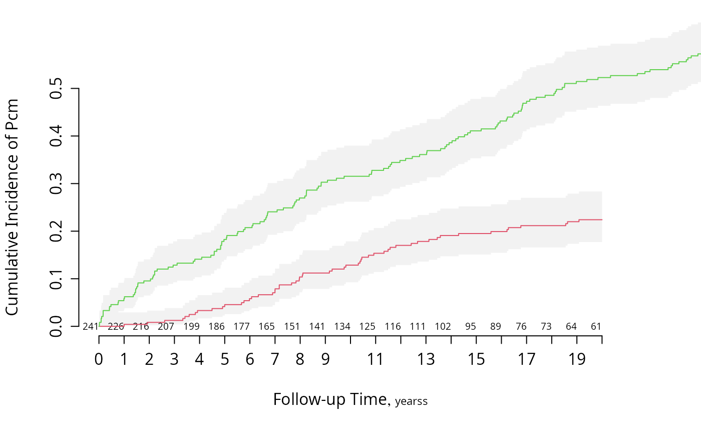
 # Use survplot for enhanced displays of cumulative incidence curves for
# competing risks
survplot(f, state='pcm', n.risk=TRUE, xlim=c(0, 20), ylim=c(0, .5), col=2)
survplot(f, state='death', add=TRUE, col=3)
# Use survplot for enhanced displays of cumulative incidence curves for
# competing risks
survplot(f, state='pcm', n.risk=TRUE, xlim=c(0, 20), ylim=c(0, .5), col=2)
survplot(f, state='death', add=TRUE, col=3)
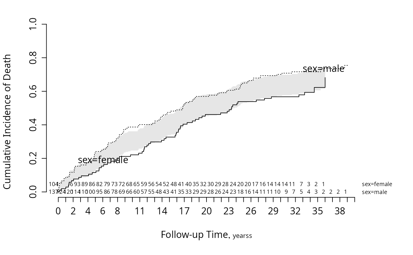
 f <- npsurv(Surv(stop, event) ~ sex, data=m)
survplot(f, state='death', n.risk=TRUE, conf='diffbands')
f <- npsurv(Surv(stop, event) ~ sex, data=m)
survplot(f, state='death', n.risk=TRUE, conf='diffbands')