Biomass Tillage Data
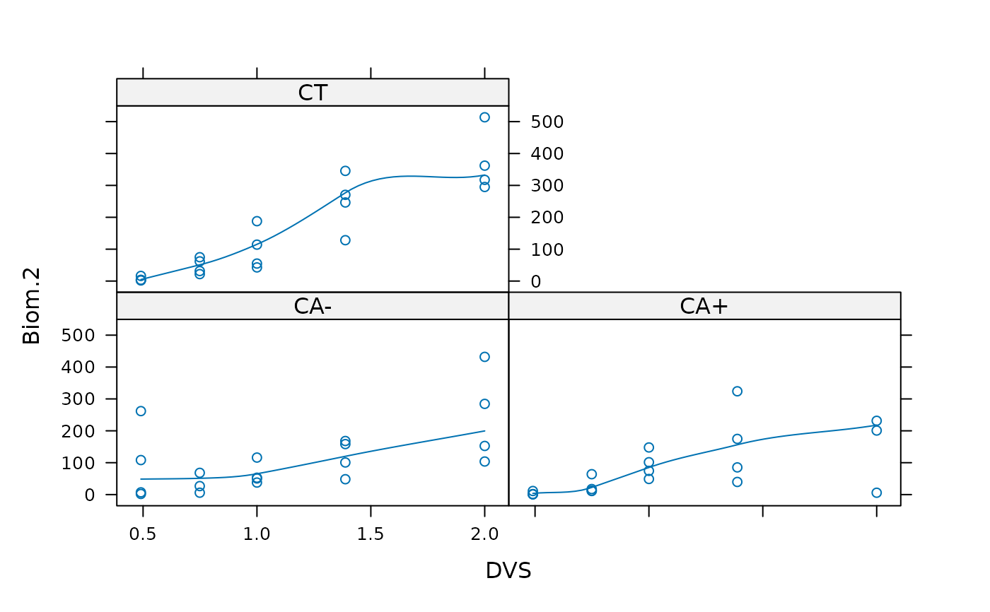
biomassTill.RdAn agricultural experiment in which different tillage methods were implemented. The effects of tillage on plant (maize) biomass were subsequently determined by modeling biomass accumulation for each tillage treatment using a 3 parameter Weibull function.
A datset where the total biomass is modeled conditional on a three value factor, and hence vector parameters are used.
data("biomassTill", package="robustbase")Format
A data frame with 58 observations on the following 3 variables.
TillageTillage treatments, a
factorwith levelsCA-:a no-tillage system with plant residues removed
CA+:a no-tillage system with plant residues retained
CT:a conventionally tilled system with residues incorporated
DVSthe development stage of the maize crop. A DVS of
1represents maize anthesis (flowering), and a DVS of2represents physiological maturity. For the data, numeric vector with 5 different values between 0.5 and 2.Biomassaccumulated biomass of maize plants from each tillage treatment.
Biom.2the same as
Biomass, but with three values replaced by “gross errors”.
Source
From Strahinja Stepanovic and John Laborde, Department of Agronomy & Horticulture, University of Nebraska-Lincoln, USA
Examples
data(biomassTill)
str(biomassTill)
#> 'data.frame': 58 obs. of 4 variables:
#> $ Tillage: Factor w/ 3 levels "CA-","CA+","CT": 1 1 1 1 1 1 1 1 1 1 ...
#> $ DVS : num 0.49 0.49 0.49 0.49 0.749 ...
#> $ Biomass: num 0.541 1.309 7.03 2.03 5.911 ...
#> $ Biom.2 : num 108.25 261.8 7.03 2.03 5.91 ...
require(lattice)
## With long tailed errors
xyplot(Biomass ~ DVS | Tillage, data = biomassTill, type=c("p","smooth"))
 ## With additional 2 outliers:
xyplot(Biom.2 ~ DVS | Tillage, data = biomassTill, type=c("p","smooth"))
## With additional 2 outliers:
xyplot(Biom.2 ~ DVS | Tillage, data = biomassTill, type=c("p","smooth"))
 ### Fit nonlinear Regression models: -----------------------------------
## simple starting values, needed:
m00st <- list(Wm = rep(300, 3),
a = rep( 1.5, 3),
b = rep( 2.2, 3))
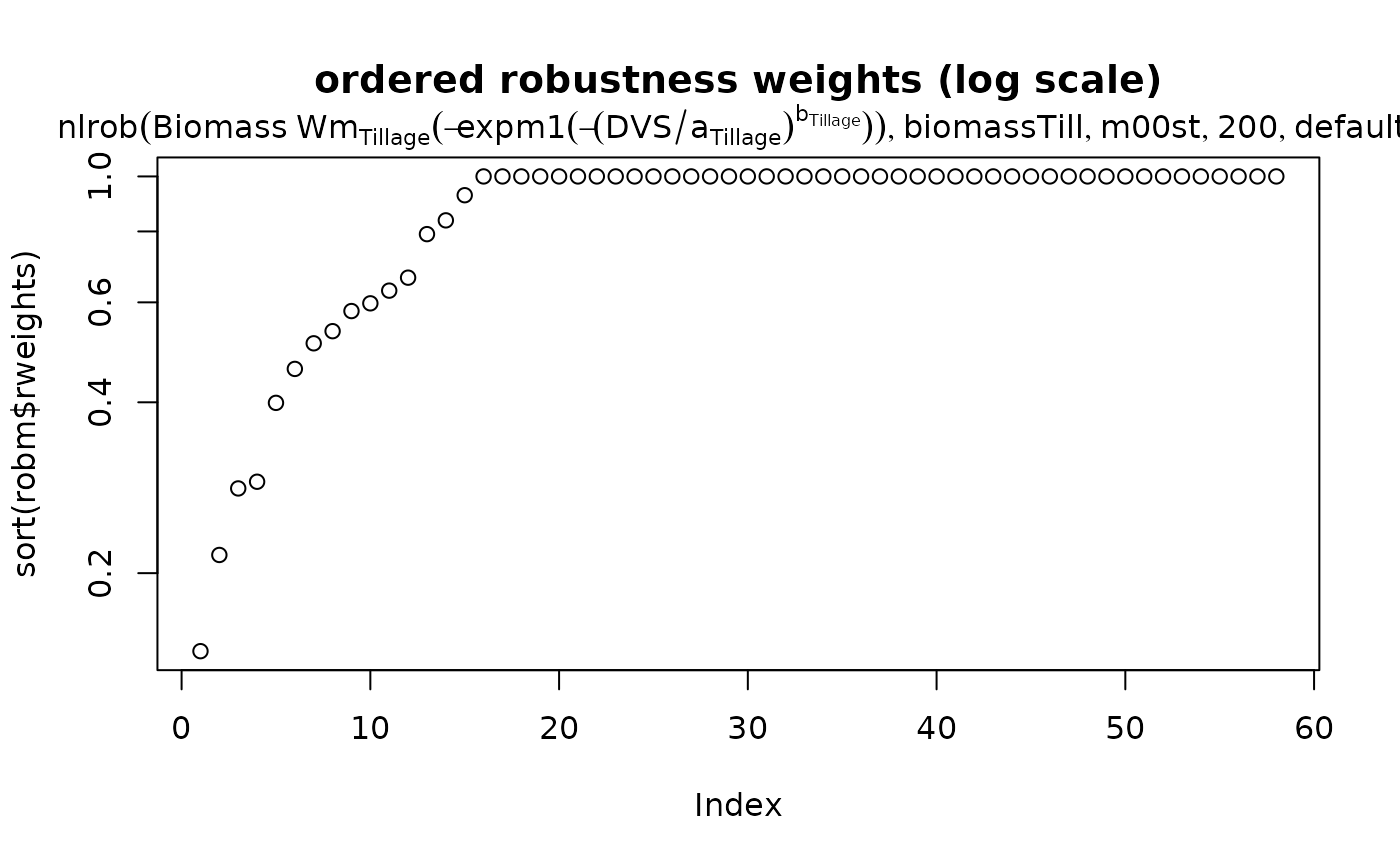
robm <- nlrob(Biomass ~ Wm[Tillage] * (-expm1(-(DVS/a[Tillage])^b[Tillage])),
data = biomassTill, start = m00st, maxit = 200)
## -----------
summary(robm) ## ... 103 IRWLS iterations
#>
#> Call:
#> nlrob(formula = Biomass ~ Wm[Tillage] * (-expm1(-(DVS/a[Tillage])^b[Tillage])),
#> data = biomassTill, start = m00st, maxit = 200, algorithm = "default")
#>
#> Residuals:
#> Min 1Q Median 3Q Max
#> -124.369 -23.776 -5.418 28.073 340.556
#>
#> Parameters:
#> Estimate Std. Error t value Pr(>|t|)
#> Wm1 219.84347 78.59343 2.797 0.007346 **
#> Wm2 265.91514 97.32363 2.732 0.008722 **
#> Wm3 343.38787 26.39224 13.011 < 2e-16 ***
#> a1 1.46076 0.41373 3.531 0.000913 ***
#> a2 1.49303 0.44386 3.364 0.001500 **
#> a3 1.29362 0.07733 16.728 < 2e-16 ***
#> b1 2.88871 1.35760 2.128 0.038409 *
#> b2 2.83763 1.18395 2.397 0.020401 *
#> b3 4.04557 0.87533 4.622 2.79e-05 ***
#> ---
#> Signif. codes: 0 ‘***’ 0.001 ‘**’ 0.01 ‘*’ 0.05 ‘.’ 0.1 ‘ ’ 1
#>
#> Robust residual standard error: 36.9
#> Convergence in 103 IRWLS iterations
#>
#> Robustness weights:
#> 43 weights are ~= 1. The remaining 15 ones are summarized as
#> Min. 1st Qu. Median Mean 3rd Qu. Max.
#> 0.1457 0.3444 0.5338 0.5237 0.6462 0.9266
plot(sort(robm$rweights), log = "y",
main = "ordered robustness weights (log scale)")
mtext(getCall(robm))
### Fit nonlinear Regression models: -----------------------------------
## simple starting values, needed:
m00st <- list(Wm = rep(300, 3),
a = rep( 1.5, 3),
b = rep( 2.2, 3))
robm <- nlrob(Biomass ~ Wm[Tillage] * (-expm1(-(DVS/a[Tillage])^b[Tillage])),
data = biomassTill, start = m00st, maxit = 200)
## -----------
summary(robm) ## ... 103 IRWLS iterations
#>
#> Call:
#> nlrob(formula = Biomass ~ Wm[Tillage] * (-expm1(-(DVS/a[Tillage])^b[Tillage])),
#> data = biomassTill, start = m00st, maxit = 200, algorithm = "default")
#>
#> Residuals:
#> Min 1Q Median 3Q Max
#> -124.369 -23.776 -5.418 28.073 340.556
#>
#> Parameters:
#> Estimate Std. Error t value Pr(>|t|)
#> Wm1 219.84347 78.59343 2.797 0.007346 **
#> Wm2 265.91514 97.32363 2.732 0.008722 **
#> Wm3 343.38787 26.39224 13.011 < 2e-16 ***
#> a1 1.46076 0.41373 3.531 0.000913 ***
#> a2 1.49303 0.44386 3.364 0.001500 **
#> a3 1.29362 0.07733 16.728 < 2e-16 ***
#> b1 2.88871 1.35760 2.128 0.038409 *
#> b2 2.83763 1.18395 2.397 0.020401 *
#> b3 4.04557 0.87533 4.622 2.79e-05 ***
#> ---
#> Signif. codes: 0 ‘***’ 0.001 ‘**’ 0.01 ‘*’ 0.05 ‘.’ 0.1 ‘ ’ 1
#>
#> Robust residual standard error: 36.9
#> Convergence in 103 IRWLS iterations
#>
#> Robustness weights:
#> 43 weights are ~= 1. The remaining 15 ones are summarized as
#> Min. 1st Qu. Median Mean 3rd Qu. Max.
#> 0.1457 0.3444 0.5338 0.5237 0.6462 0.9266
plot(sort(robm$rweights), log = "y",
main = "ordered robustness weights (log scale)")
mtext(getCall(robm))
 ## the classical (only works for the mild outliers):
cl.m <- nls(Biomass ~ Wm[Tillage] * (-expm1(-(DVS/a[Tillage])^b[Tillage])),
data = biomassTill, start = m00st)
## now for the extra-outlier data: -- fails with singular gradient !!
try(
rob2 <- nlrob(Biom.2 ~ Wm[Tillage] * (-expm1(-(DVS/a[Tillage])^b[Tillage])),
data = biomassTill, start = m00st)
)
#> Error in nls(formula, data = data, start = start, algorithm = algorithm, :
#> singular gradient
## use better starting values:
m1st <- setNames(as.list(as.data.frame(matrix(
coef(robm), 3))),
c("Wm", "a","b"))
try(# just breaks a bit later!
rob2 <- nlrob(Biom.2 ~ Wm[Tillage] * (-expm1(-(DVS/a[Tillage])^b[Tillage])),
data = biomassTill, start = m1st, maxit= 200, trace=TRUE)
)
#> robust iteration 1
#> 132570.9 (2.09e-01): par = (219.8435 265.9151 343.3879 1.460763 1.493028 1.293623 2.88871 2.837634 4.045572)
#> 128604.8 (1.33e-01): par = (256.1274 173.1572 344.2618 1.655889 1.209569 1.295166 1.999126 3.086581 4.040089)
#> 127364.3 (8.99e-02): par = (368.4797 193.1824 344.252 2.339725 1.242377 1.295119 1.649138 3.262429 4.040244)
#> 127273.3 (8.56e-02): par = (681.4524 194.0933 344.2523 4.117628 1.2451 1.29512 1.466655 3.186278 4.040239)
#> 127051.6 (7.42e-02): par = (1869.221 194.045 344.2523 10.05763 1.244583 1.29512 1.371601 3.202393 4.040239)
#> 127026.5 (7.28e-02): par = (2484.691 194.0462 344.2523 12.61518 1.244593 1.29512 1.368389 3.202187 4.040239)
#> 127020.4 (7.24e-02): par = (3015.952 194.0467 344.2523 14.67072 1.244597 1.29512 1.366951 3.202091 4.040239)
#> 127014.7 (7.21e-02): par = (3401.091 194.047 344.2523 16.08877 1.2446 1.29512 1.366276 3.202045 4.040239)
#> 127013.6 (7.20e-02): par = (3885.757 194.0473 344.2523 17.81816 1.244602 1.29512 1.365624 3.202 4.040239)
#> 127010.3 (7.18e-02): par = (4199.03 194.0474 344.2523 18.89806 1.244603 1.29512 1.365309 3.201978 4.040239)
#> 127008.1 (7.16e-02): par = (4562.638 194.0475 344.2523 20.12614 1.244604 1.29512 1.365001 3.201956 4.040239)
#> 127007.5 (7.16e-02): par = (4989.421 194.0476 344.2523 21.53651 1.244605 1.29512 1.364698 3.201935 4.040239)
#> 127005.4 (7.15e-02): par = (5243.178 194.0477 344.2523 22.35571 1.244605 1.29512 1.364549 3.201924 4.040239)
#> 127003.6 (7.14e-02): par = (5522.471 194.0478 344.2523 23.24559 1.244606 1.29512 1.364402 3.201913 4.040239)
#> 127002.2 (7.13e-02): par = (5831.268 194.0478 344.2523 24.21606 1.244606 1.29512 1.364256 3.201903 4.040239)
#> 127001.2 (7.12e-02): par = (6174.466 194.0479 344.2523 25.27927 1.244607 1.29512 1.364112 3.201892 4.040239)
#> 127000.8 (7.12e-02): par = (6558.033 194.0479 344.2523 26.44976 1.244608 1.29512 1.363969 3.201881 4.040239)
#> 126999.6 (7.11e-02): par = (6773.721 194.048 344.2523 27.09761 1.244608 1.29512 1.363898 3.201876 4.040239)
#> 126998.5 (7.10e-02): par = (7003.397 194.048 344.2523 27.78157 1.244608 1.29512 1.363828 3.201871 4.040239)
#> 126997.5 (7.10e-02): par = (7248.494 194.048 344.2523 28.50502 1.244608 1.29512 1.363758 3.201866 4.040239)
#> 126996.6 (7.09e-02): par = (7510.574 194.0481 344.2523 29.27159 1.244609 1.29512 1.363688 3.20186 4.040239)
#> 126995.8 (7.09e-02): par = (7791.469 194.0481 344.2523 30.08549 1.244609 1.29512 1.363619 3.201855 4.040239)
#> 126995.2 (7.08e-02): par = (8093.258 194.0481 344.2523 30.95147 1.244609 1.29512 1.36355 3.20185 4.040239)
#> 126994.7 (7.08e-02): par = (8418.301 194.0481 344.2523 31.87486 1.244609 1.29512 1.363482 3.201845 4.040239)
#> 126994.3 (7.08e-02): par = (8769.403 194.0482 344.2523 32.86195 1.24461 1.29512 1.363413 3.20184 4.040239)
#> 126994.2 (7.08e-02): par = (9149.77 194.0482 344.2523 33.91985 1.24461 1.29512 1.363346 3.201835 4.040239)
#> 126993.6 (7.07e-02): par = (9356.477 194.0482 344.2523 34.48835 1.24461 1.29512 1.363312 3.201832 4.040239)
#> 126993.0 (7.07e-02): par = (9572.441 194.0482 344.2523 35.0788 1.24461 1.29512 1.363278 3.201829 4.040239)
#> 126992.5 (7.07e-02): par = (9798.27 194.0483 344.2523 35.69248 1.24461 1.29512 1.363245 3.201827 4.040239)
#> 126992.0 (7.06e-02): par = (10034.67 194.0483 344.2523 36.33093 1.24461 1.29512 1.363211 3.201824 4.040239)
#> 126991.5 (7.06e-02): par = (10282.37 194.0483 344.2523 36.99568 1.24461 1.29512 1.363178 3.201822 4.040239)
#> 126991.1 (7.06e-02): par = (10542.23 194.0483 344.2523 37.68857 1.244611 1.29512 1.363144 3.201819 4.040239)
#> 126990.7 (7.06e-02): par = (10815.15 194.0483 344.2523 38.41148 1.244611 1.29512 1.363111 3.201817 4.040239)
#> 126990.4 (7.06e-02): par = (11102.13 194.0483 344.2523 39.16653 1.244611 1.29512 1.363078 3.201814 4.040239)
#> 126990.1 (7.05e-02): par = (11404.24 194.0483 344.2523 39.95586 1.244611 1.29512 1.363045 3.201812 4.040239)
#> 126989.9 (7.05e-02): par = (11722.78 194.0484 344.2523 40.78223 1.244611 1.29512 1.363012 3.201809 4.040239)
#> 126989.7 (7.05e-02): par = (12059.05 194.0484 344.2523 41.64827 1.244611 1.29512 1.362979 3.201806 4.040239)
#> 126989.6 (7.05e-02): par = (12414.59 194.0484 344.2523 42.55709 1.244611 1.29512 1.362946 3.201804 4.040239)
#> 126989.5 (7.05e-02): par = (12791.07 194.0484 344.2523 43.51207 1.244611 1.29512 1.362914 3.201801 4.040239)
#> 126989.5 (7.05e-02): par = (13190.4 194.0484 344.2523 44.51706 1.244612 1.29512 1.362881 3.201799 4.040239)
#> Error in nls(formula, data = data, start = start, algorithm = algorithm, :
#> step factor 0.000488281 reduced below 'minFactor' of 0.000976562
## Comparison {more to come} % once we have "MM" working...
rbind(start = unlist(m00st),
class = coef(cl.m),
rob = coef(robm))
#> Wm1 Wm2 Wm3 a1 a2 a3 b1 b2
#> start 300.0000 300.0000 300.0000 1.500000 1.500000 1.500000 2.200000 2.200000
#> class 489.9173 615.5279 380.0640 2.342740 2.189602 1.371278 2.397332 2.594862
#> rob 219.8435 265.9151 343.3879 1.460763 1.493028 1.293623 2.888710 2.837634
#> b3
#> start 2.200000
#> class 3.594968
#> rob 4.045572
## the classical (only works for the mild outliers):
cl.m <- nls(Biomass ~ Wm[Tillage] * (-expm1(-(DVS/a[Tillage])^b[Tillage])),
data = biomassTill, start = m00st)
## now for the extra-outlier data: -- fails with singular gradient !!
try(
rob2 <- nlrob(Biom.2 ~ Wm[Tillage] * (-expm1(-(DVS/a[Tillage])^b[Tillage])),
data = biomassTill, start = m00st)
)
#> Error in nls(formula, data = data, start = start, algorithm = algorithm, :
#> singular gradient
## use better starting values:
m1st <- setNames(as.list(as.data.frame(matrix(
coef(robm), 3))),
c("Wm", "a","b"))
try(# just breaks a bit later!
rob2 <- nlrob(Biom.2 ~ Wm[Tillage] * (-expm1(-(DVS/a[Tillage])^b[Tillage])),
data = biomassTill, start = m1st, maxit= 200, trace=TRUE)
)
#> robust iteration 1
#> 132570.9 (2.09e-01): par = (219.8435 265.9151 343.3879 1.460763 1.493028 1.293623 2.88871 2.837634 4.045572)
#> 128604.8 (1.33e-01): par = (256.1274 173.1572 344.2618 1.655889 1.209569 1.295166 1.999126 3.086581 4.040089)
#> 127364.3 (8.99e-02): par = (368.4797 193.1824 344.252 2.339725 1.242377 1.295119 1.649138 3.262429 4.040244)
#> 127273.3 (8.56e-02): par = (681.4524 194.0933 344.2523 4.117628 1.2451 1.29512 1.466655 3.186278 4.040239)
#> 127051.6 (7.42e-02): par = (1869.221 194.045 344.2523 10.05763 1.244583 1.29512 1.371601 3.202393 4.040239)
#> 127026.5 (7.28e-02): par = (2484.691 194.0462 344.2523 12.61518 1.244593 1.29512 1.368389 3.202187 4.040239)
#> 127020.4 (7.24e-02): par = (3015.952 194.0467 344.2523 14.67072 1.244597 1.29512 1.366951 3.202091 4.040239)
#> 127014.7 (7.21e-02): par = (3401.091 194.047 344.2523 16.08877 1.2446 1.29512 1.366276 3.202045 4.040239)
#> 127013.6 (7.20e-02): par = (3885.757 194.0473 344.2523 17.81816 1.244602 1.29512 1.365624 3.202 4.040239)
#> 127010.3 (7.18e-02): par = (4199.03 194.0474 344.2523 18.89806 1.244603 1.29512 1.365309 3.201978 4.040239)
#> 127008.1 (7.16e-02): par = (4562.638 194.0475 344.2523 20.12614 1.244604 1.29512 1.365001 3.201956 4.040239)
#> 127007.5 (7.16e-02): par = (4989.421 194.0476 344.2523 21.53651 1.244605 1.29512 1.364698 3.201935 4.040239)
#> 127005.4 (7.15e-02): par = (5243.178 194.0477 344.2523 22.35571 1.244605 1.29512 1.364549 3.201924 4.040239)
#> 127003.6 (7.14e-02): par = (5522.471 194.0478 344.2523 23.24559 1.244606 1.29512 1.364402 3.201913 4.040239)
#> 127002.2 (7.13e-02): par = (5831.268 194.0478 344.2523 24.21606 1.244606 1.29512 1.364256 3.201903 4.040239)
#> 127001.2 (7.12e-02): par = (6174.466 194.0479 344.2523 25.27927 1.244607 1.29512 1.364112 3.201892 4.040239)
#> 127000.8 (7.12e-02): par = (6558.033 194.0479 344.2523 26.44976 1.244608 1.29512 1.363969 3.201881 4.040239)
#> 126999.6 (7.11e-02): par = (6773.721 194.048 344.2523 27.09761 1.244608 1.29512 1.363898 3.201876 4.040239)
#> 126998.5 (7.10e-02): par = (7003.397 194.048 344.2523 27.78157 1.244608 1.29512 1.363828 3.201871 4.040239)
#> 126997.5 (7.10e-02): par = (7248.494 194.048 344.2523 28.50502 1.244608 1.29512 1.363758 3.201866 4.040239)
#> 126996.6 (7.09e-02): par = (7510.574 194.0481 344.2523 29.27159 1.244609 1.29512 1.363688 3.20186 4.040239)
#> 126995.8 (7.09e-02): par = (7791.469 194.0481 344.2523 30.08549 1.244609 1.29512 1.363619 3.201855 4.040239)
#> 126995.2 (7.08e-02): par = (8093.258 194.0481 344.2523 30.95147 1.244609 1.29512 1.36355 3.20185 4.040239)
#> 126994.7 (7.08e-02): par = (8418.301 194.0481 344.2523 31.87486 1.244609 1.29512 1.363482 3.201845 4.040239)
#> 126994.3 (7.08e-02): par = (8769.403 194.0482 344.2523 32.86195 1.24461 1.29512 1.363413 3.20184 4.040239)
#> 126994.2 (7.08e-02): par = (9149.77 194.0482 344.2523 33.91985 1.24461 1.29512 1.363346 3.201835 4.040239)
#> 126993.6 (7.07e-02): par = (9356.477 194.0482 344.2523 34.48835 1.24461 1.29512 1.363312 3.201832 4.040239)
#> 126993.0 (7.07e-02): par = (9572.441 194.0482 344.2523 35.0788 1.24461 1.29512 1.363278 3.201829 4.040239)
#> 126992.5 (7.07e-02): par = (9798.27 194.0483 344.2523 35.69248 1.24461 1.29512 1.363245 3.201827 4.040239)
#> 126992.0 (7.06e-02): par = (10034.67 194.0483 344.2523 36.33093 1.24461 1.29512 1.363211 3.201824 4.040239)
#> 126991.5 (7.06e-02): par = (10282.37 194.0483 344.2523 36.99568 1.24461 1.29512 1.363178 3.201822 4.040239)
#> 126991.1 (7.06e-02): par = (10542.23 194.0483 344.2523 37.68857 1.244611 1.29512 1.363144 3.201819 4.040239)
#> 126990.7 (7.06e-02): par = (10815.15 194.0483 344.2523 38.41148 1.244611 1.29512 1.363111 3.201817 4.040239)
#> 126990.4 (7.06e-02): par = (11102.13 194.0483 344.2523 39.16653 1.244611 1.29512 1.363078 3.201814 4.040239)
#> 126990.1 (7.05e-02): par = (11404.24 194.0483 344.2523 39.95586 1.244611 1.29512 1.363045 3.201812 4.040239)
#> 126989.9 (7.05e-02): par = (11722.78 194.0484 344.2523 40.78223 1.244611 1.29512 1.363012 3.201809 4.040239)
#> 126989.7 (7.05e-02): par = (12059.05 194.0484 344.2523 41.64827 1.244611 1.29512 1.362979 3.201806 4.040239)
#> 126989.6 (7.05e-02): par = (12414.59 194.0484 344.2523 42.55709 1.244611 1.29512 1.362946 3.201804 4.040239)
#> 126989.5 (7.05e-02): par = (12791.07 194.0484 344.2523 43.51207 1.244611 1.29512 1.362914 3.201801 4.040239)
#> 126989.5 (7.05e-02): par = (13190.4 194.0484 344.2523 44.51706 1.244612 1.29512 1.362881 3.201799 4.040239)
#> Error in nls(formula, data = data, start = start, algorithm = algorithm, :
#> step factor 0.000488281 reduced below 'minFactor' of 0.000976562
## Comparison {more to come} % once we have "MM" working...
rbind(start = unlist(m00st),
class = coef(cl.m),
rob = coef(robm))
#> Wm1 Wm2 Wm3 a1 a2 a3 b1 b2
#> start 300.0000 300.0000 300.0000 1.500000 1.500000 1.500000 2.200000 2.200000
#> class 489.9173 615.5279 380.0640 2.342740 2.189602 1.371278 2.397332 2.594862
#> rob 219.8435 265.9151 343.3879 1.460763 1.493028 1.293623 2.888710 2.837634
#> b3
#> start 2.200000
#> class 3.594968
#> rob 4.045572