Insect Damages on Carrots

The damage carrots data set from Phelps (1982) was used by McCullagh and Nelder (1989) in order to illustrate diagnostic techniques because of the presence of an outlier. In a soil experiment trial with three blocks, eight levels of insecticide were applied and the carrots were tested for insect damage.

data(carrots, package="robustbase")

Format

A data frame with 24 observations on the following 4 variables.

success

integer giving the number of carrots with insect damage.

total

integer giving the total number of carrots per experimental unit.

logdose

a numeric vector giving log(dose) values (eight different levels only).

block

factor with levels B1 to B3

Source

Phelps, K. (1982). Use of the complementary log-log function to describe doseresponse relationships in insecticide evaluation field trials.
In R. Gilchrist (Ed.), Lecture Notes in Statistics, No. 14. GLIM.82: Proceedings of the International Conference on Generalized Linear Models; Springer-Verlag.

References

McCullagh P. and Nelder, J. A. (1989) Generalized Linear Models. London: Chapman and Hall.

Eva Cantoni and Elvezio Ronchetti (2001); JASA, and
Eva Cantoni (2004); JSS, see glmrob

Examples

data(carrots)
str(carrots)
#> 'data.frame':	24 obs. of  4 variables:
#>  $ success: int  10 16 8 6 9 9 1 2 17 10 ...
#>  $ total  : int  35 42 50 42 35 42 32 28 38 40 ...
#>  $ logdose: num  1.52 1.64 1.76 1.88 2 2.12 2.24 2.36 1.52 1.64 ...
#>  $ block  : Factor w/ 3 levels "B1","B2","B3": 1 1 1 1 1 1 1 1 2 2 ...
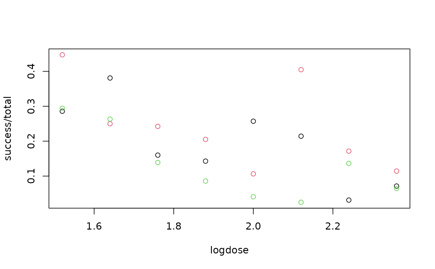
plot(success/total ~ logdose, data = carrots, col = as.integer(block))

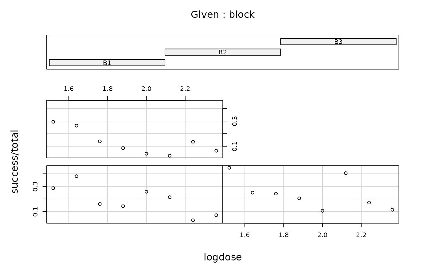
coplot(success/total ~ logdose | block, data = carrots)


## Classical glm
Cfit0 <- glm(cbind(success, total-success) ~ logdose + block,
             data=carrots, family=binomial)
summary(Cfit0)
#> 
#> Call:
#> glm(formula = cbind(success, total - success) ~ logdose + block, 
#>     family = binomial, data = carrots)
#> 
#> Coefficients:
#>             Estimate Std. Error z value Pr(>|z|)    
#> (Intercept)   2.0226     0.6501   3.111  0.00186 ** 
#> logdose      -1.8174     0.3439  -5.285 1.26e-07 ***
#> blockB2       0.3009     0.1991   1.511  0.13073    
#> blockB3      -0.5424     0.2318  -2.340  0.01929 *  
#> ---
#> Signif. codes:  0 ‘***’ 0.001 ‘**’ 0.01 ‘*’ 0.05 ‘.’ 0.1 ‘ ’ 1
#> 
#> (Dispersion parameter for binomial family taken to be 1)
#> 
#>     Null deviance: 83.344  on 23  degrees of freedom
#> Residual deviance: 39.976  on 20  degrees of freedom
#> AIC: 128.61
#> 
#> Number of Fisher Scoring iterations: 4
#> 

## Robust Fit (see help(glmrob)) ....