Robust Fitting of Generalized Linear Models
glmrob.Rdglmrob is used to fit generalized linear models by robust
methods. The models are specified by giving a symbolic description of
the linear predictor and a description of the error distribution.
Currently, robust methods are implemented for family =
binomial, = poisson, = Gamma and = gaussian.
Arguments
- formula
a
formula, i.e., a symbolic description of the model to be fit (cf.glmorlm).- family
a description of the error distribution and link function to be used in the model. This can be a character string naming a family function, a family
functionor the result of a call to a family function. (Seefamilyfor details of family functions.)- data
an optional data frame containing the variables in the model. If not found in
data, the variables are taken fromenvironment(formula), typically the environment from whichglmrobis called.- weights
an optional vector of weights to be used in the fitting process.
- subset
an optional vector specifying a subset of observations to be used in the fitting process.
- na.action
a function which indicates what should happen when the data contain
NAs. The default is set by thena.actionsetting inoptions. The “factory-fresh” default isna.omit.- start
starting values for the parameters in the linear predictor. Note that specifying
starthas somewhat different meaning for the differentmethods. Notably, for"MT", this skips the expensive computation of initial estimates via sub samples, but needs to be robust itself.- offset
this can be used to specify an a priori known component to be included in the linear predictor during fitting.
- method
a character string specifying the robust fitting method. The details of method specification are given below.
- weights.on.x
a character string (can be abbreviated), a
functionorlist(see below), or a numeric vector of lengthn, specifying how points (potential outliers) in x-space are downweighted. If"hat", weights on the design of the form \(\sqrt{1-h_{ii}}\) are used, where \(h_{ii}\) are the diagonal elements of the hat matrix. If"robCov", weights based on the robust Mahalanobis distance of the design matrix (intercept excluded) are used where the covariance matrix and the centre is estimated bycov.robfrom the package MASS.
Similarly, if"covMcd", robust weights are computed usingcovMcd. The default is"none".If
weights.on.xis afunction, it is called with arguments(X, intercept)and must return an n-vector of non-negative weights.If it is a
list, it must be of length one, and as element contain a function much likecovMcd()orcov.rob()(package MASS), which computes multivariate location and “scatter” of a data matrixX.- control
a list of parameters for controlling the fitting process. See the documentation for
glmrobMqle.controlfor details.- model
a logical value indicating whether model frame should be included as a component of the returned value.
- x, y
logical values indicating whether the response vector and model matrix used in the fitting process should be returned as components of the returned value.
- contrasts
an optional list. See the
contrasts.argofmodel.matrix.default.- trace.lev
logical (or integer) indicating if intermediate results should be printed; defaults to
0(the same asFALSE).- ...
arguments passed to
glmrobMqle.controlwhencontrolisNULL(as per default).
Details
method="model.frame" returns the model.frame(),
the same as glm().
method="Mqle" fits a generalized linear
model using Mallows or Huber type robust estimators, as described in
Cantoni and Ronchetti (2001) and Cantoni and Ronchetti (2006). In
contrast to the implementation
described in Cantoni (2004), the pure influence algorithm is
implemented.
method="WBY" and method="BY",
available for logistic regression (family = binomial) only, call
BYlogreg(*, initwml= . ) for the (weighted) Bianco-Yohai
estimator, where initwml is true for "WBY", and false
for "BY".
method="MT", currently only implemented for family = poisson,
computes an “[M]-Estimator based on [T]ransformation”,
by Valdora and Yohai (2013), via (hidden internal) glmrobMT(); as
that uses sample(), from R version 3.6.0 it depends on
RNGkind(*, sample.kind). Exact reproducibility of results
from R versions 3.5.3 and earlier, requires setting
RNGversion("3.5.0").
weights.on.x= "robCov" makes sense if all explanatory variables
are continuous.
In the cases,where weights.on.x is "covMcd" or
"robCov", or list with a “robCov” function, the
mahalanobis distances D^2 are computed with respect to the
covariance (location and scatter) estimate, and the weights are
1/sqrt(1+ pmax.int(0, 8*(D2 - p)/sqrt(2*p))),
where D2 = D^2 and p = ncol(X).
Value
glmrob returns an object of class "glmrob" and is also
inheriting from glm.
The summary method, see summary.glmrob, can
be used to obtain or print a summary of the results.
The generic accessor functions coefficients,
effects, fitted.values and residuals (see
residuals.glmrob) can be used to extract various useful
features of the value returned by glmrob().
An object of class "glmrob" is a list with at least the
following components:
- coefficients
a named vector of coefficients
- residuals
the working residuals, that is the (robustly “huberized”) residuals in the final iteration of the IWLS fit.
- fitted.values
the fitted mean values, obtained by transforming the linear predictors by the inverse of the link function.
- w.r
robustness weights for each observations; i.e.,
residuals\(\times\)w.requals the psi-function of the Preason's residuals.- w.x
weights used to down-weight observations based on the position of the observation in the design space.
- dispersion
robust estimation of dispersion paramter if appropriate
- cov
the estimated asymptotic covariance matrix of the estimated coefficients.
- tcc
the tuning constant c in Huber's psi-function.
- family
the
familyobject used.- linear.predictors
the linear fit on link scale.
- deviance
NULL; Exists because of compatipility reasons.
- iter
the number of iterations used by the influence algorithm.
- converged
logical. Was the IWLS algorithm judged to have converged?
- call
the matched call.
- formula
the formula supplied.
- terms
the
termsobject used.- data
the
data argument.- offset
the offset vector used.
- control
the value of the
controlargument used.- method
the name of the robust fitter function used.
- contrasts
(where relevant) the contrasts used.
- xlevels
(where relevant) a record of the levels of the factors used in fitting.
References
Eva Cantoni and Elvezio Ronchetti (2001) Robust Inference for Generalized Linear Models. JASA 96 (455), 1022–1030.
Eva Cantoni (2004) Analysis of Robust Quasi-deviances for Generalized Linear Models. Journal of Statistical Software, 10, https://www.jstatsoft.org/article/view/v010i04 Eva Cantoni and Elvezio Ronchetti (2006) A robust approach for skewed and heavy-tailed outcomes in the analysis of health care expenditures. Journal of Health Economics 25, 198–213.
S. Heritier, E. Cantoni, S. Copt, M.-P. Victoria-Feser (2009) Robust Methods in Biostatistics. Wiley Series in Probability and Statistics.
Marina Valdora and Víctor J. Yohai (2013) Robust estimators for Generalized Linear Models. In progress.
See also
predict.glmrob for prediction;
glmrobMqle.control
Examples
## Binomial response --------------
data(carrots)
Cfit1 <- glm(cbind(success, total-success) ~ logdose + block,
data = carrots, family = binomial)
summary(Cfit1)
#>
#> Call:
#> glm(formula = cbind(success, total - success) ~ logdose + block,
#> family = binomial, data = carrots)
#>
#> Coefficients:
#> Estimate Std. Error z value Pr(>|z|)
#> (Intercept) 2.0226 0.6501 3.111 0.00186 **
#> logdose -1.8174 0.3439 -5.285 1.26e-07 ***
#> blockB2 0.3009 0.1991 1.511 0.13073
#> blockB3 -0.5424 0.2318 -2.340 0.01929 *
#> ---
#> Signif. codes: 0 ‘***’ 0.001 ‘**’ 0.01 ‘*’ 0.05 ‘.’ 0.1 ‘ ’ 1
#>
#> (Dispersion parameter for binomial family taken to be 1)
#>
#> Null deviance: 83.344 on 23 degrees of freedom
#> Residual deviance: 39.976 on 20 degrees of freedom
#> AIC: 128.61
#>
#> Number of Fisher Scoring iterations: 4
#>
Rfit1 <- glmrob(cbind(success, total-success) ~ logdose + block,
family =
  binomial
, data = carrots, method= "Mqle",
control= glmrobMqle.control(tcc=1.2))
summary(Rfit1)
#>
#> Call: glmrob(formula = cbind(success, total - success) ~ logdose + block, family = binomial, data = carrots, method = "Mqle", control = glmrobMqle.control(tcc = 1.2))
#>
#>
#> Coefficients:
#> Estimate Std. Error z value Pr(>|z|)
#> (Intercept) 2.3883 0.6923 3.450 0.000561 ***
#> logdose -2.0491 0.3685 -5.561 2.68e-08 ***
#> blockB2 0.2351 0.2122 1.108 0.267828
#> blockB3 -0.4496 0.2409 -1.866 0.061989 .
#> ---
#> Signif. codes: 0 ‘***’ 0.001 ‘**’ 0.01 ‘*’ 0.05 ‘.’ 0.1 ‘ ’ 1
#> Robustness weights w.r * w.x:
#> 15 weights are ~= 1. The remaining 9 ones are
#> 2 5 6 7 13 14 21 22 23
#> 0.7756 0.7026 0.6751 0.9295 0.8536 0.2626 0.8337 0.9051 0.9009
#>
#> Number of observations: 24
#> Fitted by method ‘Mqle’ (in 9 iterations)
#>
#> (Dispersion parameter for binomial family taken to be 1)
#>
#> No deviance values available
#> Algorithmic parameters:
#> acc tcc
#> 0.0001 1.2000
#> maxit
#> 50
#> test.acc
#> "coef"
#>
Rfit2 <- glmrob(success/total ~ logdose + block, weights = total,
family = binomial, data = carrots, method= "Mqle",
control= glmrobMqle.control(tcc=1.2))
coef(Rfit2) ## The same as Rfit1
#> (Intercept) logdose blockB2 blockB3
#> 2.3882515 -2.0491078 0.2351038 -0.4496314
## Binary response --------------
data(vaso)
Vfit1 <- glm(Y ~ log(Volume) + log(Rate), family=binomial, data=vaso)
coef(Vfit1)
#> (Intercept) log(Volume) log(Rate)
#> -2.875422 5.179324 4.561675
Vfit2 <- glmrob(Y ~ log(Volume) + log(Rate), family=binomial, data=vaso,
method="Mqle", control = glmrobMqle.control(tcc=3.5))
coef(Vfit2) # c = 3.5 ==> not much different from classical
#> (Intercept) log(Volume) log(Rate)
#> -2.753375 4.973897 4.388113
## Note the problems with tcc <= 3 %% FIXME algorithm ???
Vfit3 <- glmrob(Y ~ log(Volume) + log(Rate), family=binomial, data=vaso,
method= "BY")
#> Convergence Achieved
coef(Vfit3)## note that results differ much.
#> (Intercept) log(Volume) log(Rate)
#> -6.851509 10.734325 9.364316
## That's not unreasonable however, see Kuensch et al.(1989), p.465
## Poisson response --------------
data(epilepsy)
Efit1 <- glm(Ysum ~ Age10 + Base4*Trt, family=poisson, data=epilepsy)
summary(Efit1)
#>
#> Call:
#> glm(formula = Ysum ~ Age10 + Base4 * Trt, family = poisson, data = epilepsy)
#>
#> Coefficients:
#> Estimate Std. Error z value Pr(>|z|)
#> (Intercept) 1.968014 0.135929 14.478 < 2e-16 ***
#> Age10 0.243490 0.041297 5.896 3.72e-09 ***
#> Base4 0.085426 0.003666 23.305 < 2e-16 ***
#> Trtprogabide -0.255257 0.076525 -3.336 0.000851 ***
#> Base4:Trtprogabide 0.007534 0.004409 1.709 0.087475 .
#> ---
#> Signif. codes: 0 ‘***’ 0.001 ‘**’ 0.01 ‘*’ 0.05 ‘.’ 0.1 ‘ ’ 1
#>
#> (Dispersion parameter for poisson family taken to be 1)
#>
#> Null deviance: 2122.73 on 58 degrees of freedom
#> Residual deviance: 556.51 on 54 degrees of freedom
#> AIC: 849.78
#>
#> Number of Fisher Scoring iterations: 5
#>
Efit2 <- glmrob(Ysum ~ Age10 + Base4*Trt, family = poisson,
data = epilepsy, method= "Mqle",
control = glmrobMqle.control(tcc= 1.2))
summary(Efit2)
#>
#> Call: glmrob(formula = Ysum ~ Age10 + Base4 * Trt, family = poisson, data = epilepsy, method = "Mqle", control = glmrobMqle.control(tcc = 1.2))
#>
#>
#> Coefficients:
#> Estimate Std. Error z value Pr(>|z|)
#> (Intercept) 2.036768 0.154168 13.211 < 2e-16 ***
#> Age10 0.158434 0.047444 3.339 0.000840 ***
#> Base4 0.085132 0.004174 20.395 < 2e-16 ***
#> Trtprogabide -0.323886 0.087421 -3.705 0.000211 ***
#> Base4:Trtprogabide 0.011842 0.004967 2.384 0.017124 *
#> ---
#> Signif. codes: 0 ‘***’ 0.001 ‘**’ 0.01 ‘*’ 0.05 ‘.’ 0.1 ‘ ’ 1
#> Robustness weights w.r * w.x:
#> 26 weights are ~= 1. The remaining 33 ones are summarized as
#> Min. 1st Qu. Median Mean 3rd Qu. Max.
#> 0.07328 0.30750 0.50730 0.49220 0.68940 0.97240
#>
#> Number of observations: 59
#> Fitted by method ‘Mqle’ (in 14 iterations)
#>
#> (Dispersion parameter for poisson family taken to be 1)
#>
#> No deviance values available
#> Algorithmic parameters:
#> acc tcc
#> 0.0001 1.2000
#> maxit
#> 50
#> test.acc
#> "coef"
#>
## 'x' weighting:
(Efit3 <- glmrob(Ysum ~ Age10 + Base4*Trt, family = poisson,
data = epilepsy, method= "Mqle", weights.on.x = "hat",
control = glmrobMqle.control(tcc= 1.2)))
#>
#> Call: glmrob(formula = Ysum ~ Age10 + Base4 * Trt, family = poisson, data = epilepsy, method = "Mqle", weights.on.x = "hat", control = glmrobMqle.control(tcc = 1.2))
#>
#> Coefficients:
#> (Intercept) Age10 Base4 Trtprogabide
#> 1.8712949 0.1898471 0.1014575 -0.2713479
#> Base4:Trtprogabide
#> 0.0007315
#>
#> Number of observations: 59
#> Fitted by method ‘Mqle’
try( # gives singular cov matrix: 'Trt' is binary factor -->
# affine equivariance and subsampling are problematic
Efit4 <- glmrob(Ysum ~ Age10 + Base4*Trt, family = poisson,
data = epilepsy, method= "Mqle", weights.on.x = "covMcd",
control = glmrobMqle.control(tcc=1.2, maxit=100))
)
#> Warning: The covariance matrix has become singular during
#> the iterations of the MCD algorithm.
#> There are 33 observations (in the entire dataset of 59 obs.) lying on
#> the hyperplane with equation a_1*(x_i1 - m_1) + ... + a_p*(x_ip - m_p)
#> = 0 with (m_1, ..., m_p) the mean of these observations and
#> coefficients a_i from the vector a <- c(0, -0.3015113, -0.904534,
#> 0.3015113)
#> Error in solve.default(cov, ...) :
#> system is computationally singular: reciprocal condition number = 5.351e-18
##--> See example(possumDiv) for another Poisson-regression
### -------- Gamma family -- data from example(glm) ---
clotting <- data.frame(
u = c(5,10,15,20,30,40,60,80,100),
lot1 = c(118,58,42,35,27,25,21,19,18),
lot2 = c(69,35,26,21,18,16,13,12,12))
summary(cl <- glm (lot1 ~ log(u), data=clotting, family=Gamma))
#>
#> Call:
#> glm(formula = lot1 ~ log(u), family = Gamma, data = clotting)
#>
#> Coefficients:
#> Estimate Std. Error t value Pr(>|t|)
#> (Intercept) -0.0165544 0.0009275 -17.85 4.28e-07 ***
#> log(u) 0.0153431 0.0004150 36.98 2.75e-09 ***
#> ---
#> Signif. codes: 0 ‘***’ 0.001 ‘**’ 0.01 ‘*’ 0.05 ‘.’ 0.1 ‘ ’ 1
#>
#> (Dispersion parameter for Gamma family taken to be 0.002446059)
#>
#> Null deviance: 3.51283 on 8 degrees of freedom
#> Residual deviance: 0.01673 on 7 degrees of freedom
#> AIC: 37.99
#>
#> Number of Fisher Scoring iterations: 3
#>
summary(ro <- glmrob(lot1 ~ log(u), data=clotting, family=Gamma))
#>
#> Call: glmrob(formula = lot1 ~ log(u), family = Gamma, data = clotting)
#>
#>
#> Coefficients:
#> Estimate Std. Error z value Pr(>|z|)
#> (Intercept) -0.0165260 0.0008369 -19.75 <2e-16 ***
#> log(u) 0.0153664 0.0003738 41.11 <2e-16 ***
#> ---
#> Signif. codes: 0 ‘***’ 0.001 ‘**’ 0.01 ‘*’ 0.05 ‘.’ 0.1 ‘ ’ 1
#> Robustness weights w.r * w.x:
#> [1] 1.0000 0.6208 1.0000 1.0000 1.0000 1.0000 1.0000 1.0000 1.0000
#>
#> Number of observations: 9
#> Fitted by method ‘Mqle’ (in 3 iterations)
#>
#> (Dispersion parameter for Gamma family taken to be 0.001869399)
#>
#> No deviance values available
#> Algorithmic parameters:
#> acc tcc
#> 0.0001 1.3450
#> maxit
#> 50
#> test.acc
#> "coef"
#>
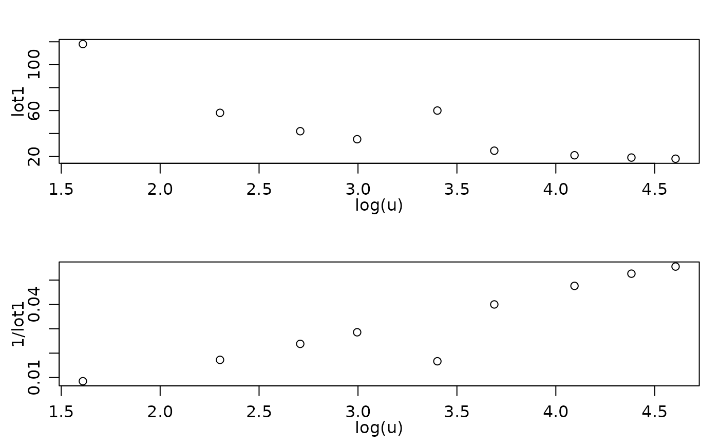
clotM5.high <- within(clotting, { lot1[5] <- 60 })
op <- par(mfrow=2:1, mgp = c(1.6, 0.8, 0), mar = c(3,3:1))
plot( lot1 ~ log(u), data=clotM5.high)
plot(1/lot1 ~ log(u), data=clotM5.high)
 par(op)
## Obviously, there the first observation is an outlier with respect to both
## representations!
cl5.high <- glm (lot1 ~ log(u), data=clotM5.high, family=Gamma)
ro5.high <- glmrob(lot1 ~ log(u), data=clotM5.high, family=Gamma)
with(ro5.high, cbind(w.x, w.r))## the 5th obs. is downweighted heavily!
#> w.x w.r
#> [1,] 1 1.00000000
#> [2,] 1 1.00000000
#> [3,] 1 1.00000000
#> [4,] 1 1.00000000
#> [5,] 1 0.07239104
#> [6,] 1 1.00000000
#> [7,] 1 1.00000000
#> [8,] 1 1.00000000
#> [9,] 1 1.00000000
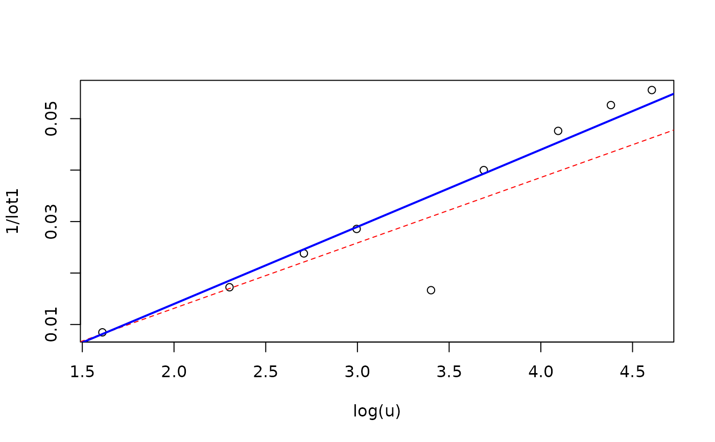
plot(1/lot1 ~ log(u), data=clotM5.high)
abline(cl5.high, lty=2, col="red")
abline(ro5.high, lwd=2, col="blue") ## result is ok (but not "perfect")
par(op)
## Obviously, there the first observation is an outlier with respect to both
## representations!
cl5.high <- glm (lot1 ~ log(u), data=clotM5.high, family=Gamma)
ro5.high <- glmrob(lot1 ~ log(u), data=clotM5.high, family=Gamma)
with(ro5.high, cbind(w.x, w.r))## the 5th obs. is downweighted heavily!
#> w.x w.r
#> [1,] 1 1.00000000
#> [2,] 1 1.00000000
#> [3,] 1 1.00000000
#> [4,] 1 1.00000000
#> [5,] 1 0.07239104
#> [6,] 1 1.00000000
#> [7,] 1 1.00000000
#> [8,] 1 1.00000000
#> [9,] 1 1.00000000
plot(1/lot1 ~ log(u), data=clotM5.high)
abline(cl5.high, lty=2, col="red")
abline(ro5.high, lwd=2, col="blue") ## result is ok (but not "perfect")