Epilepsy Attacks Data Set

Data from a clinical trial of 59 patients with epilepsy (Breslow, 1996) in order to illustrate diagnostic techniques in Poisson regression.

data(epilepsy, package="robustbase")

Format

A data frame with 59 observations on the following 11 variables.

ID

Patient identification number

Y1

Number of epilepsy attacks patients have during the first follow-up period

Y2

Number of epilepsy attacks patients have during the second follow-up period

Y3

Number of epilepsy attacks patients have during the third follow-up period

Y4

Number of epilepsy attacks patients have during the forth follow-up period

Base

Number of epileptic attacks recorded during 8 week period prior to randomization

Age

Age of the patients

Trt

a factor with levels placebo progabide indicating whether the anti-epilepsy drug Progabide has been applied or not

Ysum

Total number of epilepsy attacks patients have during the four follow-up periods

Age10

Age of the patients devided by 10

Base4

Variable Base devided by 4

Details

Thall and Vail reported data from a clinical trial of 59 patients with epilepsy, 31 of whom were randomized to receive the anti-epilepsy drug Progabide and 28 of whom received a placebo. Baseline data consisted of the patient's age and the number of epileptic seizures recorded during 8 week period prior to randomization. The response consisted of counts of seizures occuring during the four consecutive follow-up periods of two weeks each.

Source

Thall, P.F. and Vail S.C. (1990) Some covariance models for longitudinal count data with overdispersion. Biometrics 46, 657–671.

References

Diggle, P.J., Liang, K.Y., and Zeger, S.L. (1994) Analysis of Longitudinal Data; Clarendon Press.

Breslow N. E. (1996) Generalized linear models: Checking assumptions and strengthening conclusions. Statistica Applicata 8, 23–41.

Examples

data(epilepsy)
str(epilepsy)
#> 'data.frame':	59 obs. of  11 variables:
#>  $ ID   : int  104 106 107 114 116 118 123 126 130 135 ...
#>  $ Y1   : int  5 3 2 4 7 5 6 40 5 14 ...
#>  $ Y2   : int  3 5 4 4 18 2 4 20 6 13 ...
#>  $ Y3   : int  3 3 0 1 9 8 0 23 6 6 ...
#>  $ Y4   : int  3 3 5 4 21 7 2 12 5 0 ...
#>  $ Base : int  11 11 6 8 66 27 12 52 23 10 ...
#>  $ Age  : int  31 30 25 36 22 29 31 42 37 28 ...
#>  $ Trt  : Factor w/ 2 levels "placebo","progabide": 1 1 1 1 1 1 1 1 1 1 ...
#>  $ Ysum : int  14 14 11 13 55 22 12 95 22 33 ...
#>  $ Age10: num  3.1 3 2.5 3.6 2.2 2.9 3.1 4.2 3.7 2.8 ...
#>  $ Base4: num  2.75 2.75 1.5 2 16.5 6.75 3 13 5.75 2.5 ...
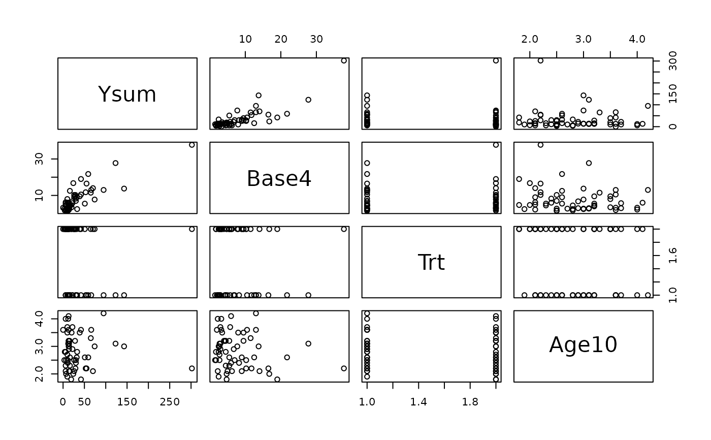
pairs(epilepsy[,c("Ysum","Base4","Trt","Age10")])


Efit1 <- glm(Ysum ~ Age10 + Base4*Trt, family=poisson, data=epilepsy)
summary(Efit1)
#> 
#> Call:
#> glm(formula = Ysum ~ Age10 + Base4 * Trt, family = poisson, data = epilepsy)
#> 
#> Coefficients:
#>                     Estimate Std. Error z value Pr(>|z|)    
#> (Intercept)         1.968014   0.135929  14.478  < 2e-16 ***
#> Age10               0.243490   0.041297   5.896 3.72e-09 ***
#> Base4               0.085426   0.003666  23.305  < 2e-16 ***
#> Trtprogabide       -0.255257   0.076525  -3.336 0.000851 ***
#> Base4:Trtprogabide  0.007534   0.004409   1.709 0.087475 .  
#> ---
#> Signif. codes:  0 ‘***’ 0.001 ‘**’ 0.01 ‘*’ 0.05 ‘.’ 0.1 ‘ ’ 1
#> 
#> (Dispersion parameter for poisson family taken to be 1)
#> 
#>     Null deviance: 2122.73  on 58  degrees of freedom
#> Residual deviance:  556.51  on 54  degrees of freedom
#> AIC: 849.78
#> 
#> Number of Fisher Scoring iterations: 5
#> 

## Robust Fit :
Efit2 <- glmrob(Ysum ~ Age10 + Base4*Trt, family=poisson, data=epilepsy,
                method = "Mqle",
                tcc=1.2, maxit=100)
summary(Efit2)
#> 
#> Call:  glmrob(formula = Ysum ~ Age10 + Base4 * Trt, family = poisson,      data = epilepsy, method = "Mqle", tcc = 1.2, maxit = 100) 
#> 
#> 
#> Coefficients:
#>                     Estimate Std. Error z value Pr(>|z|)    
#> (Intercept)         2.036768   0.154168  13.211  < 2e-16 ***
#> Age10               0.158434   0.047444   3.339 0.000840 ***
#> Base4               0.085132   0.004174  20.395  < 2e-16 ***
#> Trtprogabide       -0.323886   0.087421  -3.705 0.000211 ***
#> Base4:Trtprogabide  0.011842   0.004967   2.384 0.017124 *  
#> ---
#> Signif. codes:  0 ‘***’ 0.001 ‘**’ 0.01 ‘*’ 0.05 ‘.’ 0.1 ‘ ’ 1
#> Robustness weights w.r * w.x: 
#>  26 weights are ~= 1. The remaining 33 ones are summarized as
#>    Min. 1st Qu.  Median    Mean 3rd Qu.    Max. 
#> 0.07328 0.30750 0.50730 0.49220 0.68940 0.97240 
#> 
#> Number of observations: 59 
#> Fitted by method ‘Mqle’  (in 14 iterations)
#> 
#> (Dispersion parameter for poisson family taken to be 1)
#> 
#> No deviance values available 
#> Algorithmic parameters: 
#>    acc    tcc 
#> 0.0001 1.2000 
#> maxit 
#>   100 
#> test.acc 
#>   "coef" 
#>