Left and Right Medcouple, Robust Measures of Tail Weight

Compute the left and right ‘medcouple’, robust estimators of tail weight, in some sense robust versions of the kurtosis, the very unrobust centralized 4th moment.

lmc(x, mx = median(x, na.rm=na.rm), na.rm = FALSE, doReflect = FALSE, ...)
rmc(x, mx = median(x, na.rm=na.rm), na.rm = FALSE, doReflect = FALSE, ...)

Arguments

x

a numeric vector

mx

number, the “center” of x wrt which the left and right parts of x are defined:

    lmc(x, mx, *) :=  mc(x[x <= mx], *)
    rmc(x, mx, *) :=  mc(x[x >= mx], *)

na.rm

logical indicating how missing values (NAs) should be dealt with.

doReflect

logical indicating if mc should also be computed on the reflected sample -x. Setting doReflect=TRUE makes sense for mathematical strictness reasons, as the internal MC computes the himedian() which can differ slightly from the median. Note that mc()'s own default is true iff length(x) <= 100.

...

further arguments to mc(), see its help page.

Value

each a number (unless ... contains full.result = TRUE).

References

Brys, G., Hubert, M. and Struyf, A. (2006). Robust measures of tail weight, Computational Statistics and Data Analysis 50(3), 733–759.

and those in ‘References’ of mc.

Examples

mc(1:5)  # 0 for a symmetric sample
#> [1] 0
lmc(1:5) # 0
#> [1] 0
rmc(1:5) # 0
#> [1] 0

x1 <- c(1, 2, 7, 9, 10)
mc(x1) # = -1/3
#> [1] -0.3333333
c( lmc( x1),  lmc( x1, doReflect=TRUE))#   0  -1/3
#> [1]  0.0000000 -0.3333333
c( rmc( x1),  rmc( x1, doReflect=TRUE))# -1/3 -1/6
#> [1] -0.3333333 -0.1666667
c(-rmc(-x1), -rmc(-x1, doReflect=TRUE)) # 2/3  1/3
#> [1] 0.6666667 0.3333333

data(cushny)
lmc(cushny) # 0.2
#> [1] 0.2
rmc(cushny) # 0.45
#> [1] 0.4545455

isSym_LRmc <- function(x, tol = 1e-14)
    all.equal(lmc(-x, doReflect=TRUE),
              rmc( x, doReflect=TRUE), tolerance = tol)

sym <- c(-20, -5, -2:2, 5, 20)
stopifnot(exprs = {
    lmc(sym) == 0.5
    rmc(sym) == 0.5
    isSym_LRmc(cushny)
    isSym_LRmc(x1)
})

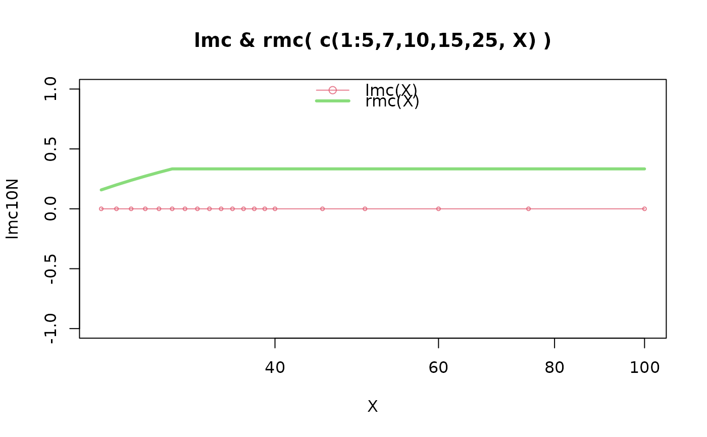
## Susceptibility to large outliers:
## "Sensitivity Curve" := empirical influence function
dX10 <- function(X) c(1:5,7,10,15,25, X) # generate skewed size-10 with 'X'
x <- c(26:40, 45, 50, 60, 75, 100)
(lmc10N <- vapply(x, function(X) lmc(dX10(X)), 1))
#>  [1] 0 0 0 0 0 0 0 0 0 0 0 0 0 0 0 0 0 0 0 0
(rmc10N <- vapply(x, function(X) rmc(dX10(X)), 1))
#>  [1] 0.1578947 0.2000000 0.2380952 0.2727273 0.3043478 0.3333333 0.3333333
#>  [8] 0.3333333 0.3333333 0.3333333 0.3333333 0.3333333 0.3333333 0.3333333
#> [15] 0.3333333 0.3333333 0.3333333 0.3333333 0.3333333 0.3333333
cols <- adjustcolor(2:3, 3/4)

plot(x, lmc10N, type="o", cex=1/2, main = "lmc & rmc( c(1:5,7,10,15,25, X) )",
     xlab=quote(X), log="x", col=cols[1])
lines(x, rmc10N, col=cols[2], lwd=3)
legend("top", paste0(c("lmc", "rmc"), "(X)"), col=cols, lty=1, lwd=c(1,3), pch = c(1, NA), bty="n")


n <- length(x)
stopifnot(exprs = {
    all.equal(current = lmc10N, target = rep(0, n))
    all.equal(current = rmc10N, target = c(3/19, 1/5, 5/21, 3/11, 7/23, rep(1/3, n-5)))
    ## and it stays stable with outlier  X --> oo :
    lmc(dX10(1e300)) == 0
    rmc(dX10(1e300)) == rmc10N[6]
})