Medcouple, a Robust Measure of Skewness

Compute the ‘medcouple’, a robust concept and estimator of skewness. The medcouple is defined as a scaled median difference of the left and right half of distribution, and hence not based on the third moment as the classical skewness.

mc(x, na.rm = FALSE, doReflect = (length(x) <= 100),
   doScale = FALSE,     # was hardwired=TRUE, then default=TRUE
   c.huberize = 1e11,   # was implicitly = Inf originally
   eps1 = 1e-14, eps2 = 1e-15,   # << new in 0.93-2 (2018-07..)
   maxit = 100, trace.lev = 0, full.result = FALSE)

Arguments

x: a numeric vector
na.rm: logical indicating how missing values (NAs) should be dealt with.
doReflect: logical indicating if the internal MC should also be computed on the reflected sample -x, with final result (mc.(x) - mc.(-x))/2. This makes sense since the internal MC, mc.() computes the himedian() which can differ slightly from the median.

doScale: logical indicating if the internal algorithm should also scale the data (using the most distant value from the median which is unrobust and numerically dangerous); scaling has been hardwired in the original algorithm and R's mc() till summer 2018, where it became the default. Since robustbase version 0.95-0, March 2022, the default is FALSE. As this may change the result, a message is printed about the new default, once per R session. You can suppress the message by specifying doScale = * explicitly, or, by setting options(mc_doScale_quiet=TRUE).
c.huberize: a positive number (default: 1e11) used to stabilize the sample via x <- huberize(x, c = c.huberize) for the mc() computations in the case of a nearly degenerate sample (many observations practically equal to the median) or very extreme outliers. In previous versions of robustbase no such huberization was applied which is equivalent to c.huberize = Inf.
eps1, eps2: tolerance in the algorithm; eps1 is used as a for convergence tolerance, where eps2 is only used in the internal h_kern() function to prevent underflow to zero, so could be considerably smaller. The original code implicitly hard coded in C eps1 := eps2 := 1e-13; only change with care!
maxit: maximal number of iterations; typically a few should be sufficient.
trace.lev: integer specifying how much diagnostic output the algorithm (in C) should produce. No output by default, most output for trace.lev = 5.
full.result: logical indicating if the full return values (from C) should be returned as a list via attr(*, "mcComp").

Value

a number between -1 and 1, which is the medcouple, \(MC(x)\). For r <- mc(x, full.result = TRUE, ....), then attr(r, "mcComp") is a list with components

medc: the medcouple \(mc.(x)\).
medc2: the medcouple \(mc.(-x)\) if doReflect=TRUE.
eps: tolerances used.
iter,iter2: number of iterations used.
converged,converged2: logical specifying “convergence”.

Convergence Problems

For extreme cases there were convergence problems which should not happen anymore as we now use doScale=FALSE and huberization (when c.huberize < Inf).

The original algorithm and mc(*, doScale=TRUE) not only centers the data around the median but also scales them by the extremes which may have a negative effect e.g., when changing an extreme outlier to even more extreme, the result changes wrongly; see the 'mc10x' example.

References

Guy Brys, Mia Hubert and Anja Struyf (2004) A Robust Measure of Skewness; JCGS 13 (4), 996–1017.

Hubert, M. and Vandervieren, E. (2008). An adjusted boxplot for skewed distributions, Computational Statistics and Data Analysis 52, 5186–5201.

Lukas Graz (2021). Improvement of the Algorithms for the Medcoule and the Adjusted Outlyingness; unpublished BSc thesis, supervised by M.Maechler, ETH Zurich.

Author

Guy Brys; modifications by Tobias Verbeke and bug fixes and extensions by Manuel Koller and Martin Maechler.

The new default doScale=FALSE, and the new c.huberize were introduced as consequence of Lukas Graz' BSc thesis.

Examples

mc(1:5) # 0 for a symmetric sample
#> [1] 0

x1 <- c(1, 2, 7, 9, 10)
mc(x1) # = -1/3
#> [1] -0.3333333

data(cushny)
mc(cushny) # 0.125
#> [1] 0.125

stopifnot(mc(c(-20, -5, -2:2, 5, 20)) == 0,
          mc(x1, doReflect=FALSE) ==  -mc(-x1, doReflect=FALSE),
          all.equal(mc(x1, doReflect=FALSE), -1/3, tolerance = 1e-12))

## Susceptibility of the current algorithm to large outliers :
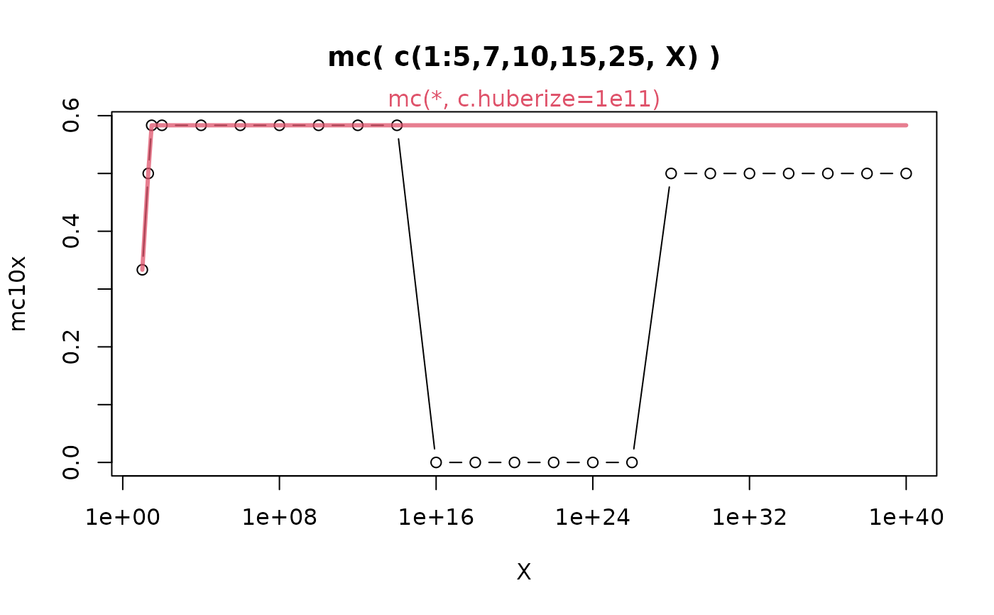
dX10 <- function(X) c(1:5,7,10,15,25, X) # generate skewed size-10 with 'X'
x <- c(10,20,30, 100^(1:20))
## (doScale=TRUE, c.huberize=Inf)  were (implicit) defaults in earlier {robustbase}:
(mc10x <- vapply(x, function(X) mc(dX10(X), doScale=TRUE, c.huberize=Inf), 1))
#>  [1] 0.3333333 0.5000000 0.5833333 0.5833333 0.5833333 0.5833333 0.5833333
#>  [8] 0.5833333 0.5833333 0.5833333 0.0000000 0.0000000 0.0000000 0.0000000
#> [15] 0.0000000 0.0000000 0.5000000 0.5000000 0.5000000 0.5000000 0.5000000
#> [22] 0.5000000 0.5000000
## limit X -> Inf  should be 7/12 = 0.58333...  but that "breaks down a bit" :
plot(x, mc10x, type="b", main = "mc( c(1:5,7,10,15,25, X) )", xlab="X", log="x")
## The new behavior is much preferable {shows message about new 'doScale=FALSE'}:
(mc10N <- vapply(x, function(X) mc(dX10(X)), 1))
#>  [1] 0.3333333 0.5000000 0.5833333 0.5833333 0.5833333 0.5833333 0.5833333
#>  [8] 0.5833333 0.5833333 0.5833333 0.5833333 0.5833333 0.5833333 0.5833333
#> [15] 0.5833333 0.5833333 0.5833333 0.5833333 0.5833333 0.5833333 0.5833333
#> [22] 0.5833333 0.5833333
lines(x, mc10N, col=adjustcolor(2, 3/4), lwd=3)
mtext("mc(*, c.huberize=1e11)",  col=2)

stopifnot(all.equal(c(4, 6, rep(7, length(x)-2))/12, mc10N))
## Here, huberization already solves the issue:
mc10NS <- vapply(x, function(X) mc(dX10(X), doScale=TRUE), 1)
stopifnot(all.equal(mc10N, mc10NS))