Robust Regression Outlier Statistics

Simple statistics about observations with robustness weight of almost zero for models that include factor terms. The number of rejected observations and the mean robustness weights are computed for each level of each factor included in the model.

outlierStats(object, x = object$x, control = object$control
           , epsw = control$eps.outlier
           , epsx = control$eps.x
           , warn.limit.reject = control$warn.limit.reject
           , warn.limit.meanrw = control$warn.limit.meanrw
           , shout = NA)

Arguments

object: object of class "lmrob", typically the result of a call to lmrob.
x: design matrix
control: list as returned by lmrob.control().
epsw: limit on the robustness weight below which an observation is considered to be an outlier. Either a numeric(1) or a function that takes the number of observations as an argument.
epsx: limit on the absolute value of the elements of the design matrix below which an element is considered zero. Either a numeric(1) or a function that takes the maximum absolute value in the design matrix as an argument.
warn.limit.reject: limit of ratio \(\#\mbox{rejected} / \#\mbox{obs in level}\) above (\(\geq\)) which a warning is produced. Set to NULL to disable warning.
warn.limit.meanrw: limit of the mean robustness per factor level below which (\(\leq\)) a warning is produced. Set to NULL to disable warning.
shout: a logical (scalar) indicating if large "Ratio" or small "Mean.RobWeight" should lead to corresponding warning()s; cutoffs are determined by warn.limit.reject and warn.limit.meanrw, above. By default, NA; setting it to FALSE or TRUE disables or unconditionally enables “shouting”.

Details

For models that include factors, the fast S-algorithm used by lmrob can produce “bad” fits for some of the factor levels, especially if there are many levels with only a few observations. Such a “bad” fit is characterized as a fit where most of the observations in a level of a factor are rejected, i.e., are assigned robustness weights of zero or nearly zero. We call such a fit a “local exact fit”.

If a local exact fit is detected, then we recommend to increase some of the control parameters of the “fast S”-algorithm. As a first aid solution in such cases, one can use setting="KS2014", see also lmrob.control.

This function is called internally by lmrob to issue a warning if a local exact fit is detected. The output is available as ostats in objects of class "lmrob" (only if the statistic is computed).

Value

A data frame for each column with any zero elements as well as an overall statistic. The data frame consist of the names of the coefficients in question, the number of non-zero observations in that level (N.nonzero), the number of rejected observations (N.rejected), the ratio of rejected observations to the number of observations in that level (Ratio) and the mean robustness weight of all the observations in the corresponding level (Mean.RobWeight).

References

Koller, M. and Stahel, W.A. (2017) Nonsingular subsampling for regression S estimators with categorical predictors, Computational Statistics 32(2): 631–646. doi:10.1007/s00180-016-0679-x

Author

Manuel Koller

Examples

## artificial data example
data <- expand.grid(grp1 = letters[1:5], grp2 = letters[1:5], rep=1:3)
set.seed(101)
data$y <- c(rt(nrow(data), 1))
## compute outlier statistics for all the estimators
control <- lmrob.control(method = "SMDM",
                         compute.outlier.stats = c("S", "MM", "SMD", "SMDM"))
## warning is only issued for some seeds
set.seed(2)
fit1 <- lmrob(y ~ grp1*grp2, data, control = control)
#> Warning: Detected possible local breakdown of S-estimate in coefficient 'grp1c:grp2c'.
#> Use lmrob argument 'setting="KS2014"' to avoid this problem.
## do as suggested:
fit2 <- lmrob(y ~ grp1*grp2, data, setting = "KS2014")

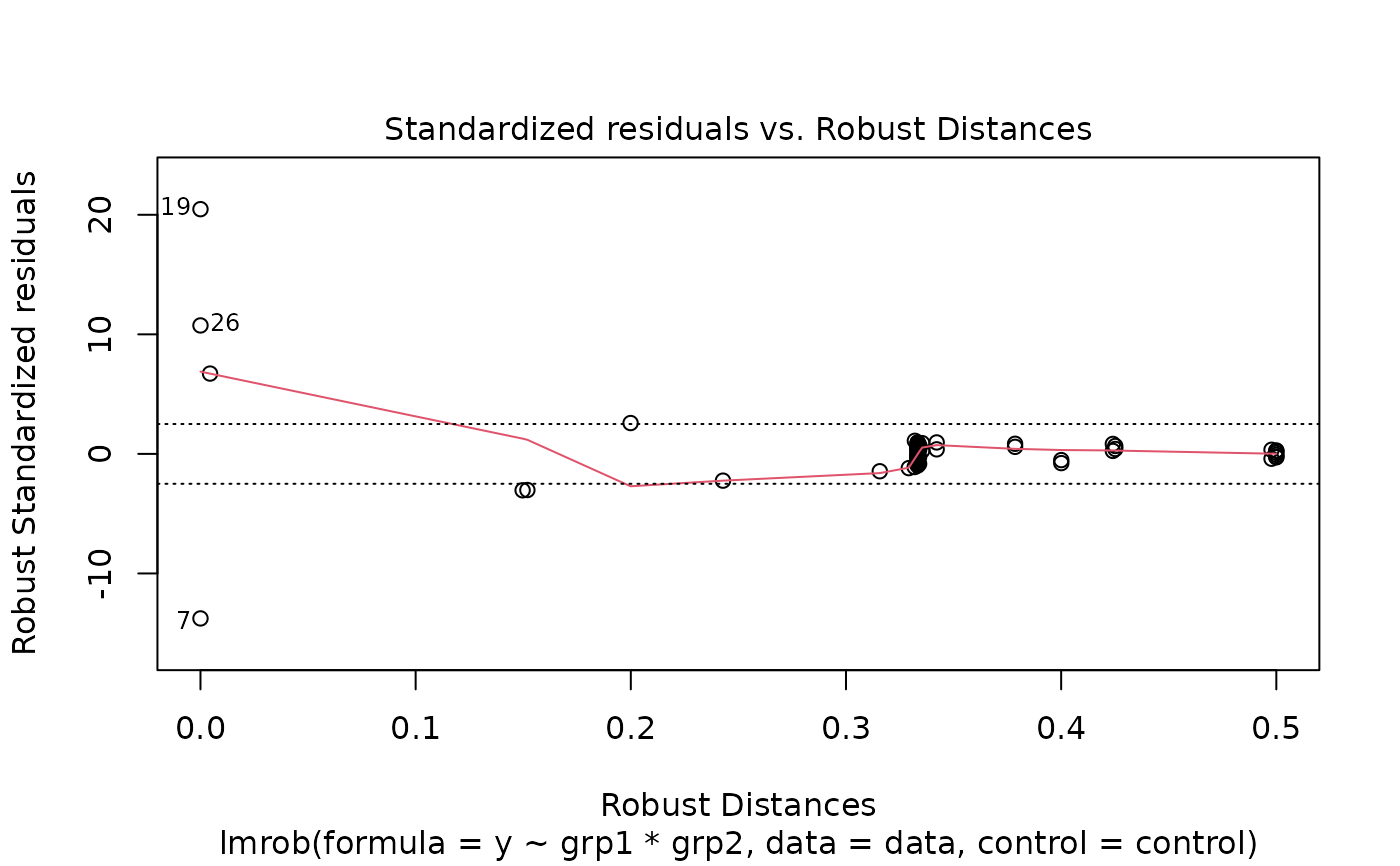
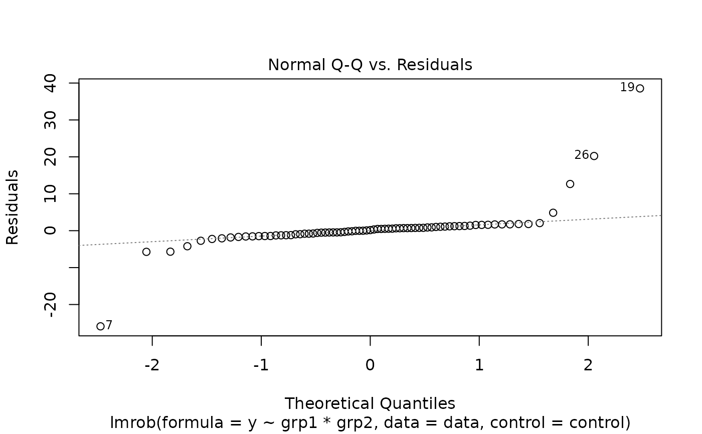
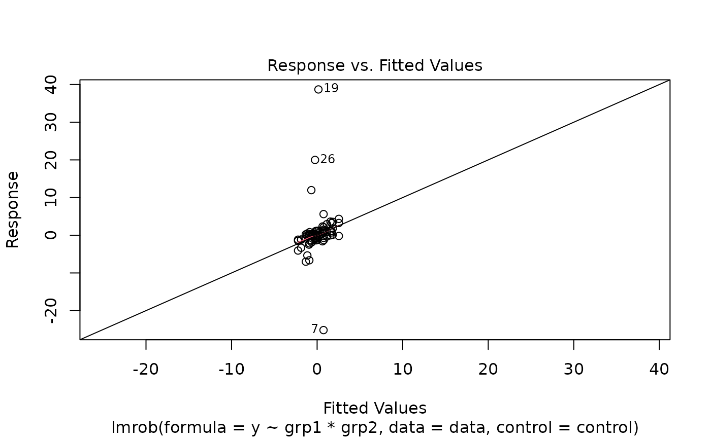
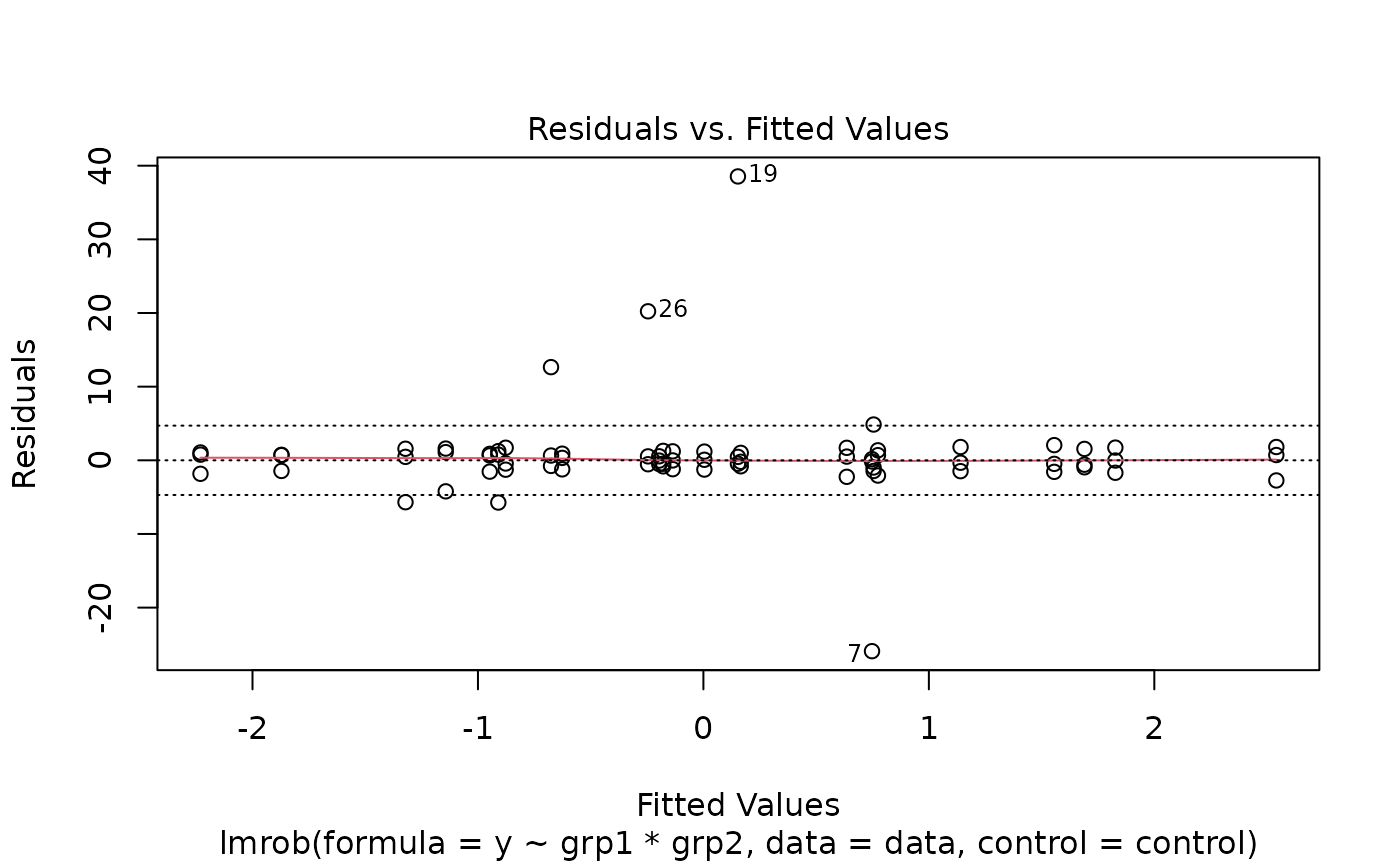
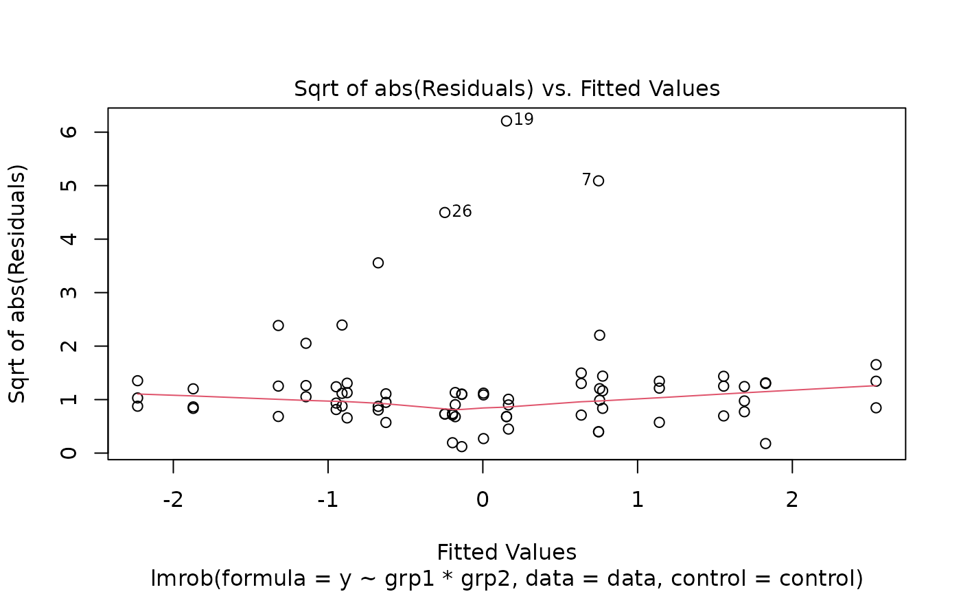
## the plot function should work for such models as well
plot(fit1)
#> recomputing robust Mahalanobis distances
#> Warning: Failed to compute robust Mahalanobis distances, reverting to robust leverages.






if (FALSE) { # \dontrun{
  ## access statistics:
  fit1$ostats ## SMDM
  fit1$init$ostats ## SMD
  fit1$init$init$ostats ## SM
  fit1$init$init$init.S$ostats ## S
} # }