MM-type Estimators for Linear Regression
lmrob.RdComputes fast MM-type estimators for linear (regression) models.
lmrob(formula, data, subset, weights, na.action, method = "MM",
      model = TRUE, x = !control$compute.rd, y = FALSE,
      singular.ok = TRUE, contrasts = NULL, offset = NULL,
      control = NULL, init = NULL, ...)
Arguments
- formula
a symbolic description of the model to be fit. See
lmandformulafor more details.- data
an optional data frame, list or environment (or object coercible by
as.data.frameto a data frame) containing the variables in the model. If not found indata, the variables are taken fromenvironment(formula), typically the environment from whichlmrobis called.- subset
an optional vector specifying a subset of observations to be used in the fitting process.
- weights
an optional vector of weights to be used in the fitting process (in addition to the robustness weights computed in the fitting process).
- na.action
a function which indicates what should happen when the data contain
NAs. The default is set by thena.actionsetting ofoptions, and isna.failif that is unset. The “factory-fresh” default isna.omit. Another possible value isNULL, no action. Valuena.excludecan be useful.- method
string specifying the estimator-chain.
MMis interpreted asSM. See Details, notably the currently recommendedsetting = "KS2014".- model, x, y
logicals. If
TRUEthe corresponding components of the fit (the model frame, the model matrix, the response) are returned.- singular.ok
logical. If
FALSE(the default in S but not in R) a singular fit is an error.- contrasts
an optional list. See the
contrasts.argofmodel.matrix.default.- offset
this can be used to specify an a priori known component to be included in the linear predictor during fitting. An
offsetterm can be included in the formula instead or as well, and if both are specified their sum is used.- control
a
listspecifying control parameters; use the functionlmrob.control(.)and see its help page.- init
an optional argument to specify or supply the initial estimate. See Details.
- ...
additional arguments can be used to specify control parameters directly instead of (but not in addition to!) via
control.
Details
- Overview:
This function computes an MM-type regression estimator as described in Yohai (1987) and Koller and Stahel (2011). By default it uses a bi-square redescending score function, and it returns a highly robust and highly efficient estimator (with 50% breakdown point and 95% asymptotic efficiency for normal errors). The computation is carried out by a call to
lmrob.fit().The argument
settingoflmrob.controlis provided to set alternative defaults as suggested in Koller and Stahel (2011) (setting="KS2011"; now do use its extensionsetting="KS2014"). For further details, seelmrob.control.- Initial Estimator
init: The initial estimator may be specified using the argument
init. This can either bea string used to specify built in internal estimators (currently
"S"and"M-S", see See also below);a
functiontaking argumentsx, y, control, mf(wheremfstands formodel.frame) and returning alistcontaining at least the initial coefficients as component"coefficients"and the initial scale estimate as"scale".Or a
listgiving the initial coefficients and scale as components"coefficients"and"scale". See also Examples.
Note that when
initis a function or list, themethodargument must not contain the initial estimator, e.g., useMDMinstead ofSMDM.The default, equivalent to
init = "S", uses as initial estimator an S-estimator (Rousseeuw and Yohai, 1984) which is computed using the Fast-S algorithm of Salibian-Barrera and Yohai (2006), callinglmrob.S(). That function, since March 2012, by default uses nonsingular subsampling which makes the Fast-S algorithm feasible for categorical data as well, see Koller (2012). Note that convergence problems may still show up as warnings, e.g.,S refinements did not converge (to refine.tol=1e-07) in 200 (= k.max) stepsand often can simply be remedied by increasing (i.e. weakening)
refine.tolor increasing the allowed number of iterationsk.max, seelmrob.control.- Method
method: The following chain of estimates is customizable via the
methodargument. There are currently two types of estimates available,"M":corresponds to the standard M-regression estimate.
"D":stands for the Design Adaptive Scale estimate as proposed in Koller and Stahel (2011).
The
methodargument takes a string that specifies the estimates to be calculated as a chain. Settingmethod='SMDM'will result in an intial S-estimate, followed by an M-estimate, a Design Adaptive Scale estimate and a final M-step. For methods involving aD-step, the default value ofpsi(seelmrob.control) is changed to"lqq".By default, standard errors are computed using the formulas of Croux, Dhaene and Hoorelbeke (2003) (
lmrob.controloptioncov=".vcov.avar1"). This method, however, works only for MM-estimates (i.e.,method = "MM"or= "SM"). For othermethodarguments, the covariance matrix estimate used is based on the asymptotic normality of the estimated coefficients (cov=".vcov.w") as described in Koller and Stahel (2011). The var-cov computation can be skipped bycov = "none"and (re)done later by e.g.,vcov(<obj>, cov = ".vcov.w").As of robustbase version 0.91-0 (April 2014), the computation of robust standard errors for
method="SMDM"has been changed. The old behaviour can be restored by setting the control parametercov.corrfact = "tauold".
Value
An object of class lmrob; a list including the following
components:
- coefficients
The estimate of the coefficient vector
- scale
The scale as used in the M estimator.
- residuals
Residuals associated with the estimator.
- converged
TRUEif the IRWLS iterations have converged.- iter
number of IRWLS iterations
- rweights
the “robustness weights” \(\psi(r_i/S) / (r_i/S)\).
- fitted.values
Fitted values associated with the estimator.
- init.S
The
listreturned bylmrob.S()orlmrob.M.S()(for MM-estimates, i.e.,method="MM"or"SM"only)- init
A similar list that contains the results of intermediate estimates (not for MM-estimates).
- rank
the numeric rank of the fitted linear model.
- cov
The estimated covariance matrix of the regression coefficients
- df.residual
the residual degrees of freedom.
- weights
the specified weights (missing if none were used).
- na.action
(where relevant) information returned by
model.frameon the special handling ofNAs.- offset
the offset used (missing if none were used).
- contrasts
(only where relevant) the contrasts used.
- xlevels
(only where relevant) a record of the levels of the factors used in fitting.
- call
the matched call.
- terms
the
termsobject used.
- model
if requested (the default), the model frame used.
- x
if requested, the model matrix used.
- y
if requested, the response used.
In addition, non-null fits will have components assign,
and qr relating to the linear fit, for use by extractor
functions such as summary.
References
Croux, C., Dhaene, G. and Hoorelbeke, D. (2003) Robust standard errors for robust estimators, Discussion Papers Series 03.16, K.U. Leuven, CES.
Koller, M. (2012)
Nonsingular subsampling for S-estimators with categorical predictors,
ArXiv e-prints https://arxiv.org/abs/1208.5595;
extended version published as Koller and Stahel (2017), see
lmrob.control.
Koller, M. and Stahel, W.A. (2011) Sharpening Wald-type inference in robust regression for small samples. Computational Statistics & Data Analysis 55(8), 2504–2515.
Maronna, R. A., and Yohai, V. J. (2000) Robust regression with both continuous and categorical predictors. Journal of Statistical Planning and Inference 89, 197–214.
Rousseeuw, P.J. and Yohai, V.J. (1984) Robust regression by means of S-estimators, In Robust and Nonlinear Time Series, J. Franke, W. Härdle and R. D. Martin (eds.). Lectures Notes in Statistics 26, 256–272, Springer Verlag, New York.
Salibian-Barrera, M. and Yohai, V.J. (2006) A fast algorithm for S-regression estimates, Journal of Computational and Graphical Statistics 15(2), 414–427. doi:10.1198/106186006X113629
Yohai, V.J. (1987) High breakdown-point and high efficiency estimates for regression. The Annals of Statistics 15, 642–65.
Yohai, V., Stahel, W.~A. and Zamar, R. (1991) A procedure for robust estimation and inference in linear regression; in Stahel and Weisberg (eds), Directions in Robust Statistics and Diagnostics, Part II, Springer, New York, 365–374; doi:10.1007/978-1-4612-4444-8_20 .
See also
lmrob.control;
for the algorithms lmrob.S, lmrob.M.S and
lmrob.fit;
and for methods,
summary.lmrob, for the extra “statistics”,
notably \(R^2\) (“R squared”);
predict.lmrob,
print.lmrob, plot.lmrob, and
weights.lmrob.
Examples
data(coleman)
set.seed(0)
## Default for a very long time:
summary( m1 <- lmrob(Y ~ ., data=coleman) )
#>
#> Call:
#> lmrob(formula = Y ~ ., data = coleman)
#> \--> method = "MM"
#> Residuals:
#> Min 1Q Median 3Q Max
#> -4.16181 -0.39226 0.01611 0.55619 7.22766
#>
#> Coefficients:
#> Estimate Std. Error t value Pr(>|t|)
#> (Intercept) 30.50232 6.71260 4.544 0.000459 ***
#> salaryP -1.66615 0.43129 -3.863 0.001722 **
#> fatherWc 0.08425 0.01467 5.741 5.10e-05 ***
#> sstatus 0.66774 0.03385 19.726 1.30e-11 ***
#> teacherSc 1.16778 0.10983 10.632 4.35e-08 ***
#> motherLev -4.13657 0.92084 -4.492 0.000507 ***
#> ---
#> Signif. codes: 0 ‘***’ 0.001 ‘**’ 0.01 ‘*’ 0.05 ‘.’ 0.1 ‘ ’ 1
#>
#> Robust residual standard error: 1.134
#> Multiple R-squared: 0.9814, Adjusted R-squared: 0.9747
#> Convergence in 11 IRWLS iterations
#>
#> Robustness weights:
#> observation 18 is an outlier with |weight| = 0 ( < 0.005);
#> The remaining 19 ones are summarized as
#> Min. 1st Qu. Median Mean 3rd Qu. Max.
#> 0.1491 0.9412 0.9847 0.9279 0.9947 0.9982
#> Algorithmic parameters:
#> tuning.chi bb tuning.psi refine.tol
#> 1.548e+00 5.000e-01 4.685e+00 1.000e-07
#> rel.tol scale.tol solve.tol zero.tol
#> 1.000e-07 1.000e-10 1.000e-07 1.000e-10
#> eps.outlier eps.x warn.limit.reject warn.limit.meanrw
#> 5.000e-03 1.569e-10 5.000e-01 5.000e-01
#> nResample max.it best.r.s k.fast.s k.max
#> 500 50 2 1 200
#> maxit.scale trace.lev mts compute.rd fast.s.large.n
#> 200 0 1000 0 2000
#> psi subsampling cov
#> "bisquare" "nonsingular" ".vcov.avar1"
#> compute.outlier.stats
#> "SM"
#> seed : int(0)
## Nowadays **strongly recommended** for routine use:
summary(m2 <- lmrob(Y ~ ., data=coleman, setting = "KS2014") )
#>
#> Call:
#> lmrob(formula = Y ~ ., data = coleman, setting = "KS2014")
#> \--> method = "SMDM"
#> Residuals:
#> Min 1Q Median 3Q Max
#> -4.18529 -0.42074 0.02314 0.55263 7.22731
#>
#> Coefficients:
#> Estimate Std. Error t value Pr(>|t|)
#> (Intercept) 30.43635 6.07018 5.014 0.000190 ***
#> salaryP -1.67840 0.51387 -3.266 0.005628 **
#> fatherWc 0.08504 0.02286 3.719 0.002287 **
#> sstatus 0.66706 0.04203 15.869 2.41e-10 ***
#> teacherSc 1.17113 0.18062 6.484 1.44e-05 ***
#> motherLev -4.13766 0.93212 -4.439 0.000561 ***
#> ---
#> Signif. codes: 0 ‘***’ 0.001 ‘**’ 0.01 ‘*’ 0.05 ‘.’ 0.1 ‘ ’ 1
#>
#> Robust residual standard error: 0.9746
#> Multiple R-squared: 0.982, Adjusted R-squared: 0.9755
#> Convergence in 7 IRWLS iterations
#>
#> Robustness weights:
#> observation 18 is an outlier with |weight| <= 0.0012 ( < 0.005);
#> 16 weights are ~= 1. The remaining 3 ones are
#> 3 16 17
#> 0.1368 0.9955 0.9755
#> Algorithmic parameters:
#> tuning.chi1 tuning.chi2 tuning.chi3 tuning.chi4
#> -5.000e-01 1.500e+00 NA 5.000e-01
#> bb tuning.psi1 tuning.psi2 tuning.psi3
#> 5.000e-01 -5.000e-01 1.500e+00 9.500e-01
#> tuning.psi4 refine.tol rel.tol scale.tol
#> NA 1.000e-07 1.000e-07 1.000e-10
#> solve.tol zero.tol eps.outlier eps.x
#> 1.000e-07 1.000e-10 5.000e-03 1.569e-10
#> warn.limit.reject warn.limit.meanrw
#> 5.000e-01 5.000e-01
#> nResample max.it best.r.s k.fast.s k.max
#> 1000 500 20 2 2000
#> maxit.scale trace.lev mts compute.rd numpoints
#> 200 0 1000 0 10
#> fast.s.large.n
#> 2000
#> setting psi subsampling
#> "KS2014" "lqq" "nonsingular"
#> cov compute.outlier.stats
#> ".vcov.w" "SMDM"
#> seed : int(0)
## ------------------
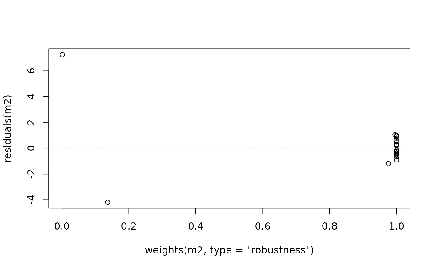
plot(residuals(m2) ~ weights(m2, type="robustness")) ##-> weights.lmrob()
abline(h=0, lty=3)
 data(starsCYG, package = "robustbase")
## Plot simple data and fitted lines
plot(starsCYG)
lmST <- lm(log.light ~ log.Te, data = starsCYG)
(RlmST <- lmrob(log.light ~ log.Te, data = starsCYG))
#>
#> Call:
#> lmrob(formula = log.light ~ log.Te, data = starsCYG)
#> \--> method = "MM"
#> Coefficients:
#> (Intercept) log.Te
#> -4.969 2.253
#>
abline(lmST, col = "red")
abline(RlmST, col = "blue")
data(starsCYG, package = "robustbase")
## Plot simple data and fitted lines
plot(starsCYG)
lmST <- lm(log.light ~ log.Te, data = starsCYG)
(RlmST <- lmrob(log.light ~ log.Te, data = starsCYG))
#>
#> Call:
#> lmrob(formula = log.light ~ log.Te, data = starsCYG)
#> \--> method = "MM"
#> Coefficients:
#> (Intercept) log.Te
#> -4.969 2.253
#>
abline(lmST, col = "red")
abline(RlmST, col = "blue")
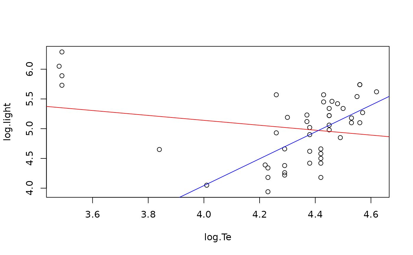 ## --> Least Sq.:/ negative slope \ robust: slope ~= 2.2 % checked in ../tests/lmrob-data.R
summary(RlmST) # -> 4 outliers; rest perfect
#>
#> Call:
#> lmrob(formula = log.light ~ log.Te, data = starsCYG)
#> \--> method = "MM"
#> Residuals:
#> Min 1Q Median 3Q Max
#> -0.80959 -0.28838 0.00282 0.36668 3.39585
#>
#> Coefficients:
#> Estimate Std. Error t value Pr(>|t|)
#> (Intercept) -4.9694 3.4100 -1.457 0.15198
#> log.Te 2.2532 0.7691 2.930 0.00531 **
#> ---
#> Signif. codes: 0 ‘***’ 0.001 ‘**’ 0.01 ‘*’ 0.05 ‘.’ 0.1 ‘ ’ 1
#>
#> Robust residual standard error: 0.4715
#> Multiple R-squared: 0.3737, Adjusted R-squared: 0.3598
#> Convergence in 15 IRWLS iterations
#>
#> Robustness weights:
#> 4 observations c(11,20,30,34) are outliers with |weight| = 0 ( < 0.0021);
#> 4 weights are ~= 1. The remaining 39 ones are summarized as
#> Min. 1st Qu. Median Mean 3rd Qu. Max.
#> 0.6533 0.9171 0.9593 0.9318 0.9848 0.9986
#> Algorithmic parameters:
#> tuning.chi bb tuning.psi refine.tol
#> 1.548e+00 5.000e-01 4.685e+00 1.000e-07
#> rel.tol scale.tol solve.tol zero.tol
#> 1.000e-07 1.000e-10 1.000e-07 1.000e-10
#> eps.outlier eps.x warn.limit.reject warn.limit.meanrw
#> 2.128e-03 8.404e-12 5.000e-01 5.000e-01
#> nResample max.it best.r.s k.fast.s k.max
#> 500 50 2 1 200
#> maxit.scale trace.lev mts compute.rd fast.s.large.n
#> 200 0 1000 0 2000
#> psi subsampling cov
#> "bisquare" "nonsingular" ".vcov.avar1"
#> compute.outlier.stats
#> "SM"
#> seed : int(0)
vcov(RlmST)
#> (Intercept) log.Te
#> (Intercept) 11.628338 -2.6221417
#> log.Te -2.622142 0.5914543
#> attr(,"weights")
#> 1 2 3 4 5 6 7 8
#> 0.9495503 0.9239441 0.9632237 0.9239441 0.9112033 0.9415944 0.6532507 0.9986423
#> 9 10 11 12 13 14 15 16
#> 0.6700018 0.9759260 0.0000000 0.9229432 0.9645902 0.9998978 0.9233596 0.9324119
#> 17 18 19 20 21 22 23 24
#> 0.8479334 0.7493654 0.9412319 0.0000000 0.9593133 0.9090245 0.8714281 0.9640937
#> 25 26 27 28 29 30 31 32
#> 0.9940525 0.9559661 0.9994487 0.9999999 0.9909255 0.0000000 0.9079843 0.9828421
#> 33 34 35 36 37 38 39 40
#> 0.9891620 0.0000000 0.9799916 0.9867941 0.9922722 0.9891620 0.9986483 0.8764843
#> 41 42 43 44 45 46 47
#> 0.9682416 0.9999967 0.9881656 0.9674794 0.9730027 0.9975596 0.9041552
#> attr(,"eigen")
#> eigen() decomposition
#> $values
#> [1] 1.221963e+01 1.639891e-04
#>
#> $vectors
#> [,1] [,2]
#> [1,] -0.9755054 -0.2199755
#> [2,] 0.2199755 -0.9755054
#>
stopifnot(all.equal(fitted(RlmST),
predict(RlmST, newdata = starsCYG), tol = 1e-14))
## FIXME: setting = "KS2011" or setting = "KS2014" **FAIL** here
##--- 'init' argument -----------------------------------
## 1) string
set.seed(0)
m3 <- lmrob(Y ~ ., data=coleman, init = "S")
stopifnot(all.equal(m1[-18], m3[-18]))
## 2) function
initFun <- function(x, y, control, ...) { # no 'mf' needed
init.S <- lmrob.S(x, y, control)
list(coefficients=init.S$coef, scale = init.S$scale)
}
set.seed(0)
m4 <- lmrob(Y ~ ., data=coleman, method = "M", init = initFun)
## list
m5 <- lmrob(Y ~ ., data=coleman, method = "M",
init = list(coefficients = m3$init$coef, scale = m3$scale))
stopifnot(all.equal(m4[-17], m5[-17]))
## --> Least Sq.:/ negative slope \ robust: slope ~= 2.2 % checked in ../tests/lmrob-data.R
summary(RlmST) # -> 4 outliers; rest perfect
#>
#> Call:
#> lmrob(formula = log.light ~ log.Te, data = starsCYG)
#> \--> method = "MM"
#> Residuals:
#> Min 1Q Median 3Q Max
#> -0.80959 -0.28838 0.00282 0.36668 3.39585
#>
#> Coefficients:
#> Estimate Std. Error t value Pr(>|t|)
#> (Intercept) -4.9694 3.4100 -1.457 0.15198
#> log.Te 2.2532 0.7691 2.930 0.00531 **
#> ---
#> Signif. codes: 0 ‘***’ 0.001 ‘**’ 0.01 ‘*’ 0.05 ‘.’ 0.1 ‘ ’ 1
#>
#> Robust residual standard error: 0.4715
#> Multiple R-squared: 0.3737, Adjusted R-squared: 0.3598
#> Convergence in 15 IRWLS iterations
#>
#> Robustness weights:
#> 4 observations c(11,20,30,34) are outliers with |weight| = 0 ( < 0.0021);
#> 4 weights are ~= 1. The remaining 39 ones are summarized as
#> Min. 1st Qu. Median Mean 3rd Qu. Max.
#> 0.6533 0.9171 0.9593 0.9318 0.9848 0.9986
#> Algorithmic parameters:
#> tuning.chi bb tuning.psi refine.tol
#> 1.548e+00 5.000e-01 4.685e+00 1.000e-07
#> rel.tol scale.tol solve.tol zero.tol
#> 1.000e-07 1.000e-10 1.000e-07 1.000e-10
#> eps.outlier eps.x warn.limit.reject warn.limit.meanrw
#> 2.128e-03 8.404e-12 5.000e-01 5.000e-01
#> nResample max.it best.r.s k.fast.s k.max
#> 500 50 2 1 200
#> maxit.scale trace.lev mts compute.rd fast.s.large.n
#> 200 0 1000 0 2000
#> psi subsampling cov
#> "bisquare" "nonsingular" ".vcov.avar1"
#> compute.outlier.stats
#> "SM"
#> seed : int(0)
vcov(RlmST)
#> (Intercept) log.Te
#> (Intercept) 11.628338 -2.6221417
#> log.Te -2.622142 0.5914543
#> attr(,"weights")
#> 1 2 3 4 5 6 7 8
#> 0.9495503 0.9239441 0.9632237 0.9239441 0.9112033 0.9415944 0.6532507 0.9986423
#> 9 10 11 12 13 14 15 16
#> 0.6700018 0.9759260 0.0000000 0.9229432 0.9645902 0.9998978 0.9233596 0.9324119
#> 17 18 19 20 21 22 23 24
#> 0.8479334 0.7493654 0.9412319 0.0000000 0.9593133 0.9090245 0.8714281 0.9640937
#> 25 26 27 28 29 30 31 32
#> 0.9940525 0.9559661 0.9994487 0.9999999 0.9909255 0.0000000 0.9079843 0.9828421
#> 33 34 35 36 37 38 39 40
#> 0.9891620 0.0000000 0.9799916 0.9867941 0.9922722 0.9891620 0.9986483 0.8764843
#> 41 42 43 44 45 46 47
#> 0.9682416 0.9999967 0.9881656 0.9674794 0.9730027 0.9975596 0.9041552
#> attr(,"eigen")
#> eigen() decomposition
#> $values
#> [1] 1.221963e+01 1.639891e-04
#>
#> $vectors
#> [,1] [,2]
#> [1,] -0.9755054 -0.2199755
#> [2,] 0.2199755 -0.9755054
#>
stopifnot(all.equal(fitted(RlmST),
predict(RlmST, newdata = starsCYG), tol = 1e-14))
## FIXME: setting = "KS2011" or setting = "KS2014" **FAIL** here
##--- 'init' argument -----------------------------------
## 1) string
set.seed(0)
m3 <- lmrob(Y ~ ., data=coleman, init = "S")
stopifnot(all.equal(m1[-18], m3[-18]))
## 2) function
initFun <- function(x, y, control, ...) { # no 'mf' needed
init.S <- lmrob.S(x, y, control)
list(coefficients=init.S$coef, scale = init.S$scale)
}
set.seed(0)
m4 <- lmrob(Y ~ ., data=coleman, method = "M", init = initFun)
## list
m5 <- lmrob(Y ~ ., data=coleman, method = "M",
init = list(coefficients = m3$init$coef, scale = m3$scale))
stopifnot(all.equal(m4[-17], m5[-17]))