Pension Funds Data
pension.RdThe total 1981 premium income of pension funds of Dutch firms, for 18 Professional Branches, from de Wit (1982).
data(pension, package="robustbase")Format
A data frame with 18 observations on the following 2 variables.
IncomePremium Income (in millions of guilders)
ReservesPremium Reserves (in millions of guilders)
Source
P. J. Rousseeuw and A. M. Leroy (1987) Robust Regression and Outlier Detection; Wiley, p.76, table 13.
Examples
data(pension)
plot(pension)
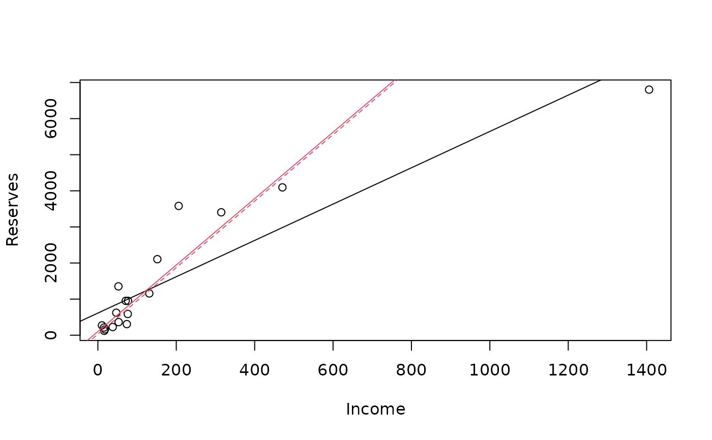
summary(lm.p <- lm(Reserves ~., data=pension))
#>
#> Call:
#> lm(formula = Reserves ~ ., data = pension)
#>
#> Residuals:
#> Min 1Q Median 3Q Max
#> -886.3 -533.5 -309.6 352.8 1931.4
#>
#> Coefficients:
#> Estimate Std. Error t value Pr(>|t|)
#> (Intercept) 613.0206 216.6178 2.830 0.0121 *
#> Income 5.0316 0.5916 8.505 2.48e-07 ***
#> ---
#> Signif. codes: 0 ‘***’ 0.001 ‘**’ 0.01 ‘*’ 0.05 ‘.’ 0.1 ‘ ’ 1
#>
#> Residual standard error: 801.2 on 16 degrees of freedom
#> Multiple R-squared: 0.8189, Adjusted R-squared: 0.8076
#> F-statistic: 72.34 on 1 and 16 DF, p-value: 2.483e-07
#>
summary(lmR.p <- lmrob(Reserves ~., data=pension))
#>
#> Call:
#> lmrob(formula = Reserves ~ ., data = pension)
#> \--> method = "MM"
#> Residuals:
#> Min 1Q Median 3Q Max
#> -6245.07 -223.74 -69.83 180.69 1580.51
#>
#> Coefficients:
#> Estimate Std. Error t value Pr(>|t|)
#> (Intercept) 103.9083 97.5007 1.066 0.302
#> Income 9.2042 0.9429 9.761 3.84e-08 ***
#> ---
#> Signif. codes: 0 ‘***’ 0.001 ‘**’ 0.01 ‘*’ 0.05 ‘.’ 0.1 ‘ ’ 1
#>
#> Robust residual standard error: 352.9
#> Multiple R-squared: 0.9156, Adjusted R-squared: 0.9103
#> Convergence in 10 IRWLS iterations
#>
#> Robustness weights:
#> observation 18 is an outlier with |weight| = 0 ( < 0.0056);
#> one weight is ~= 1. The remaining 16 ones are summarized as
#> Min. 1st Qu. Median Mean 3rd Qu. Max.
#> 0.007457 0.873200 0.964300 0.863500 0.986100 0.996200
#> Algorithmic parameters:
#> tuning.chi bb tuning.psi refine.tol
#> 1.548e+00 5.000e-01 4.685e+00 1.000e-07
#> rel.tol scale.tol solve.tol zero.tol
#> 1.000e-07 1.000e-10 1.000e-07 1.000e-10
#> eps.outlier eps.x warn.limit.reject warn.limit.meanrw
#> 5.556e-03 2.558e-09 5.000e-01 5.000e-01
#> nResample max.it best.r.s k.fast.s k.max
#> 500 50 2 1 200
#> maxit.scale trace.lev mts compute.rd fast.s.large.n
#> 200 0 1000 0 2000
#> psi subsampling cov
#> "bisquare" "nonsingular" ".vcov.avar1"
#> compute.outlier.stats
#> "SM"
#> seed : int(0)
summary(lts.p <- ltsReg(Reserves ~., data=pension))
#>
#> Call:
#> ltsReg.formula(formula = Reserves ~ ., data = pension)
#>
#> Residuals (from reweighted LS):
#> Min 1Q Median 3Q Max
#> -404.1 -129.2 0.0 199.6 839.9
#>
#> Coefficients:
#> Estimate Std. Error t value Pr(>|t|)
#> Intercept 30.7415 119.5759 0.257 0.801
#> Income 9.2091 0.7627 12.074 8.64e-09 ***
#> ---
#> Signif. codes: 0 ‘***’ 0.001 ‘**’ 0.01 ‘*’ 0.05 ‘.’ 0.1 ‘ ’ 1
#>
#> Residual standard error: 365.7 on 14 degrees of freedom
#> Multiple R-Squared: 0.9124, Adjusted R-squared: 0.9061
#> F-statistic: 145.8 on 1 and 14 DF, p-value: 8.641e-09
#>
abline( lm.p)
abline(lmR.p, col=2)
abline(lts.p, col=2, lty=2)
 ## MM: "the" solution is much simpler:
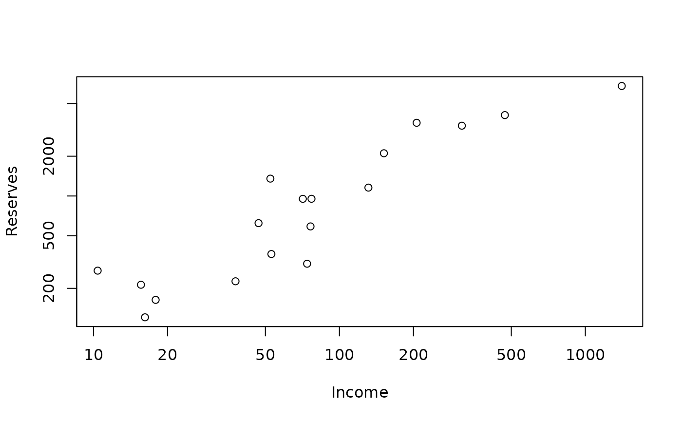
plot(pension, log = "xy")
## MM: "the" solution is much simpler:
plot(pension, log = "xy")
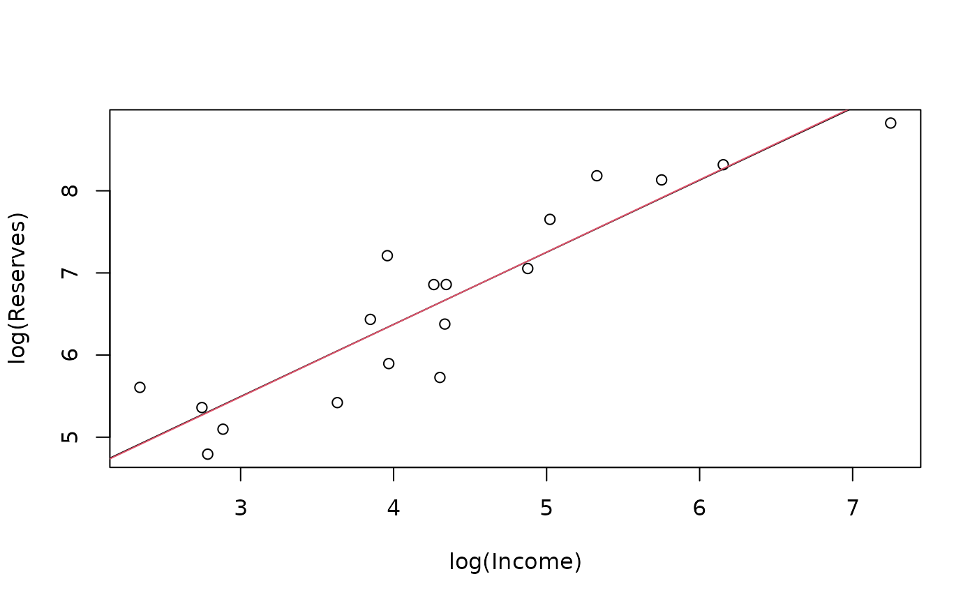
 lm.lp <- lm(log(Reserves) ~ log(Income), data=pension)
lmR.lp <- lmrob(log(Reserves) ~ log(Income), data=pension)
plot(log(Reserves) ~ log(Income), data=pension)
## no difference between LS and robust:
abline( lm.lp)
abline(lmR.lp, col=2)
lm.lp <- lm(log(Reserves) ~ log(Income), data=pension)
lmR.lp <- lmrob(log(Reserves) ~ log(Income), data=pension)
plot(log(Reserves) ~ log(Income), data=pension)
## no difference between LS and robust:
abline( lm.lp)
abline(lmR.lp, col=2)