Plot Method for "lmrob" Objects

Diagnostic plots for elements of class lmrob

# S3 method for class 'lmrob'
plot(x, which = 1:5,
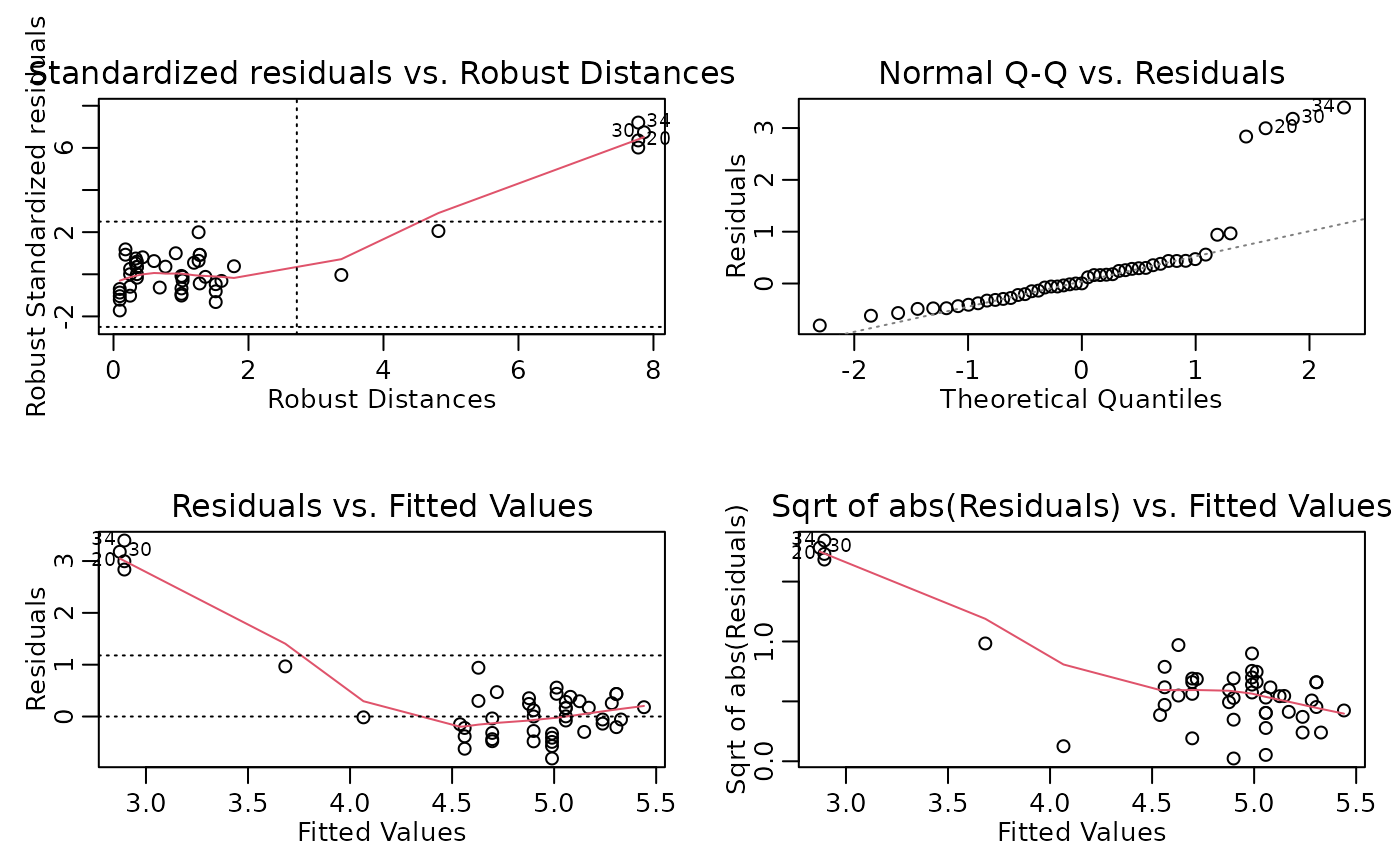
     caption = c("Standardized residuals vs. Robust Distances",
   "Normal Q-Q vs. Residuals", "Response vs. Fitted Values",
   "Residuals vs. Fitted Values" , "Sqrt of abs(Residuals) vs. Fitted Values"),
   panel = if(add.smooth) panel.smooth else points,
   sub.caption = deparse(x$call), main = "",
   compute.MD = TRUE,
   ask = prod(par("mfcol")) < length(which) && dev.interactive(),
   id.n = 3, labels.id = names(residuals(x)), cex.id = 0.75,
   label.pos = c(4,2), qqline = TRUE, add.smooth = getOption("add.smooth"),
   ..., p=0.025)

Arguments

x

an object as created by lmrob

which

integer number between 1 and 5 to specify which plot is desired

caption

Caption for the different plots

panel

panel function. The useful alternative to points, panel.smooth can be chosen by add.smooth = TRUE.

main

main title

sub.caption

sub titles

compute.MD

logical indicating if the robust Mahalanobis distances should be recomputed, using covMcd() when needed, i.e., if which contains 1.

ask

waits for user input before displaying each plot

id.n

number of points to be labelled in each plot, starting with the most extreme.

labels.id

vector of labels, from which the labels for extreme points will be chosen. NULL uses observation numbers.

cex.id

magnification of point labels.

label.pos

positioning of labels, for the left half and right half of the graph respectively.

qqline

logical indicating if a qqline() should be added to the normal Q-Q plot.

add.smooth

logical indicating if a smoother should be added to most plots; see also panel above.

...

optional arguments for par, title, etc.

p

threshold for distance-distance plot

References

Robust diagnostic plots as in Rousseeuw and van Zomeren (1990), see ‘References’ in ltsPlot.

Details

if compute.MD = TRUE and the robust Mahalanobis distances need to be computed, they are stored (“cached”) with the object x when this function has been called from top-level.

See also

lmrob, also for examples, plot.lm.

Examples

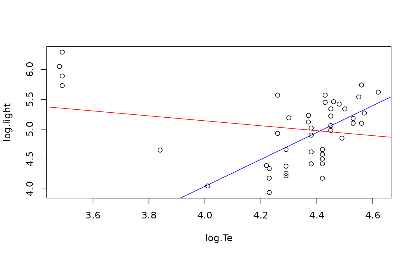
data(starsCYG)
## Plot simple data and fitted lines
plot(starsCYG)
 lmST <-    lm(log.light ~ log.Te, data = starsCYG)
RlmST <- lmrob(log.light ~ log.Te, data = starsCYG)
RlmST
#> 
#> Call:
#> lmrob(formula = log.light ~ log.Te, data = starsCYG)
#>  \--> method = "MM"
#> Coefficients:
#> (Intercept)       log.Te  
#>      -4.969        2.253  
#> 
abline(lmST, col = "red")
abline(RlmST, col = "blue")


op <- par(mfrow = c(2,2), mgp = c(1.5, 0.6, 0), mar= .1+c(3,3,3,1))
plot(RlmST, which = c(1:2, 4:5))
#> recomputing robust Mahalanobis distances

par(op)