Predict method for Robust Linear Model ("lmrob") Fits
predict.lmrob.RdPredicted values based on robust linear model object.
Arguments
- object
object of class inheriting from
"lmrob"- newdata
an optional data frame in which to look for variables with which to predict. If omitted, the fitted values are used.
- se.fit
a switch indicating if standard errors are required.
- scale
scale parameter for std.err. calculation
- df
degrees of freedom for scale
- interval
type of interval calculation.
- level
tolerance/confidence level
- type
Type of prediction (response or model term).
- terms
if
type="terms", which terms (default is all terms)- na.action
function determining what should be done with missing values in
newdata. The default is to predictNA.- pred.var
the variance(s) for future observations to be assumed for prediction intervals. See ‘Details’.
- weights
variance weights for prediction. This can be a numeric vector or a one-sided model formula. In the latter case, it is interpreted as an expression evaluated in
newdata- ...
further arguments passed to or from other methods.
Details
Note that this lmrob method for predict is
closely modeled after the method for lm(),
predict.lm, maybe see there for caveats with missing
value treatment.
The prediction intervals are for a single observation at each case in
newdata (or by default, the data used for the fit) with error
variance(s) pred.var. This can be a multiple of res.var,
the estimated value of \(\sigma^2\): the default is to assume that
future observations have the same error variance as those
used for fitting. If weights is supplied, the inverse of this
is used as a scale factor. For a weighted fit, if the prediction
is for the original data frame, weights defaults to the weights
used for the model fit, with a warning since it might not be the
intended result. If the fit was weighted and newdata is given, the
default is to assume constant prediction variance, with a warning.
Value
predict.lmrob produces a vector of predictions or a matrix of
predictions and bounds with column names fit, lwr, and
upr if interval is set. If se.fit is
TRUE, a list with the following components is returned:
- fit
vector or matrix as above
- se.fit
standard error of predicted means
- residual.scale
residual standard deviations
- df
degrees of freedom for residual
See also
lmrob and the (non-robust) traditional
predict.lm method.
Examples
## Predictions --- artificial example -- closely following example(predict.lm)
set.seed(5)
n <- length(x <- sort(c(round(rnorm(25), 1), 20)))
y <- x + rnorm(n)
iO <- c(sample(n-1, 3), n)
y[iO] <- y[iO] + 10*rcauchy(iO)
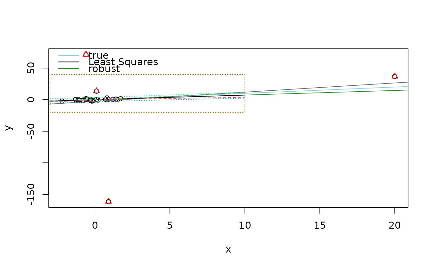
p.ex <- function(...) {
plot(y ~ x, ...); abline(0,1, col="sky blue")
points(y ~ x, subset=iO, col="red", pch=2)
abline(lm (y ~ x), col = "gray40")
abline(lmrob(y ~ x), col = "forest green")
legend("topleft", c("true", "Least Squares", "robust"),
col = c("sky blue", "gray40", "forest green"), lwd=1.5, bty="n")
}
p.ex()
fm <- lmrob(y ~ x)
predict(fm)
#> 1 2 3 4 5 6
#> -1.59670367 -0.94084168 -0.79509457 -0.79509457 -0.57647390 -0.57647390
#> 7 8 9 10 11 12
#> -0.43072680 -0.43072680 -0.43072680 -0.35785324 -0.21210613 -0.21210613
#> 13 14 15 16 17 18
#> -0.13923258 -0.06635902 0.07938809 0.07938809 0.15226164 0.51662941
#> 19 20 21 22 23 24
#> 0.58950297 0.66237652 0.66237652 0.88099719 1.02674430 1.09961785
#> 25 26
#> 1.24536496 14.58122544
new <- data.frame(x = seq(-3, 10, 0.25))
str(predict(fm, new, se.fit = TRUE))
#> List of 4
#> $ fit : Named num [1:53] -2.18 -2 -1.82 -1.63 -1.45 ...
#> ..- attr(*, "names")= chr [1:53] "1" "2" "3" "4" ...
#> $ se.fit : Named num [1:53] 0.671 0.628 0.586 0.545 0.504 ...
#> ..- attr(*, "names")= chr [1:53] "1" "2" "3" "4" ...
#> $ df : int 24
#> $ residual.scale: num 1.66
pred.w.plim <- predict(fm, new, interval = "prediction")
pred.w.clim <- predict(fm, new, interval = "confidence")
pmat <- cbind(pred.w.clim, pred.w.plim[,-1])
matlines(new$x, pmat, lty = c(1,2,2,3,3))# add to first plot
## show zoom-in region :
rect(xleft = -3, ybottom = -20, xright = 10, ytop = 40,
lty = 3, border="orange4")
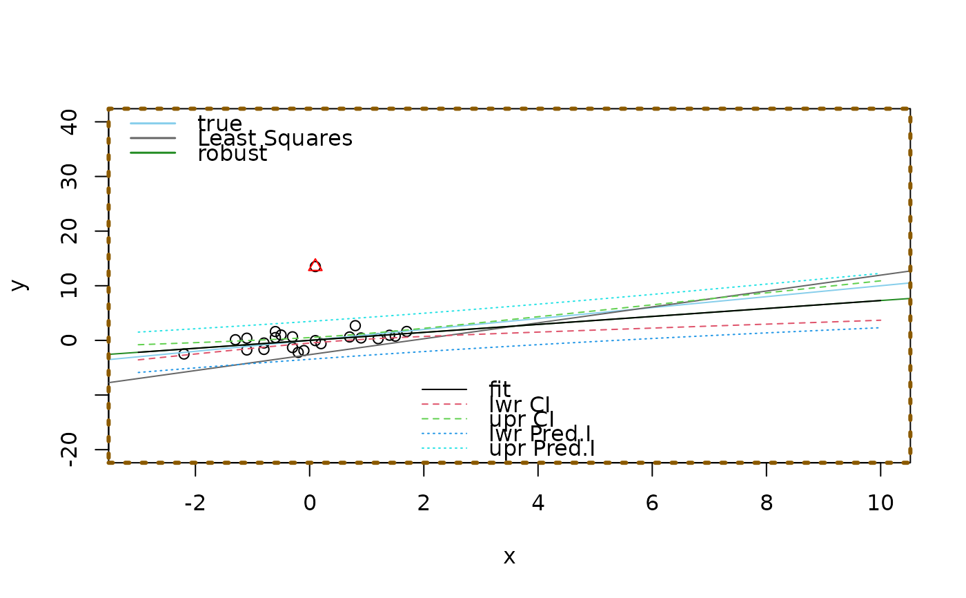
 ## now zoom in :
p.ex(xlim = c(-3,10), ylim = c(-20, 40))
matlines(new$x, pmat, lty = c(1,2,2,3,3))
box(lty = 3, col="orange4", lwd=3)
legend("bottom", c("fit", "lwr CI", "upr CI", "lwr Pred.I", "upr Pred.I"),
col = 1:5, lty=c(1,2,2,3,3), bty="n")
## now zoom in :
p.ex(xlim = c(-3,10), ylim = c(-20, 40))
matlines(new$x, pmat, lty = c(1,2,2,3,3))
box(lty = 3, col="orange4", lwd=3)
legend("bottom", c("fit", "lwr CI", "upr CI", "lwr Pred.I", "upr Pred.I"),
col = 1:5, lty=c(1,2,2,3,3), bty="n")
 ## Prediction intervals, special cases
## The first three of these throw warnings
w <- 1 + x^2
fit <- lmrob(y ~ x)
wfit <- lmrob(y ~ x, weights = w)
predict(fit, interval = "prediction")
#> Warning: Predictions on current data refer to _future_ responses
#> fit lwr upr
#> 1 -1.59670367 -5.198296 2.004889
#> 2 -0.94084168 -4.463549 2.581865
#> 3 -0.79509457 -4.304443 2.714254
#> 4 -0.79509457 -4.304443 2.714254
#> 5 -0.57647390 -4.068711 2.915763
#> 6 -0.57647390 -4.068711 2.915763
#> 7 -0.43072680 -3.913529 3.052076
#> 8 -0.43072680 -3.913529 3.052076
#> 9 -0.43072680 -3.913529 3.052076
#> 10 -0.35785324 -3.836536 3.120829
#> 11 -0.21210613 -3.683750 3.259537
#> 12 -0.21210613 -3.683750 3.259537
#> 13 -0.13923258 -3.607960 3.329495
#> 14 -0.06635902 -3.532573 3.399855
#> 15 0.07938809 -3.383014 3.541790
#> 16 0.07938809 -3.383014 3.541790
#> 17 0.15226164 -3.308842 3.613366
#> 18 0.51662941 -2.944081 3.977339
#> 19 0.58950297 -2.872348 4.051353
#> 20 0.66237652 -2.801020 4.125773
#> 21 0.66237652 -2.801020 4.125773
#> 22 0.88099719 -2.589468 4.351462
#> 23 1.02674430 -2.450448 4.503937
#> 24 1.09961785 -2.381540 4.580775
#> 25 1.24536496 -2.244918 4.735648
#> 26 14.58122544 6.479946 22.682505
predict(wfit, interval = "prediction")
#> Warning: Predictions on current data refer to _future_ responses
#> Warning: Assuming prediction variance inversely proportional to weights used for fitting
#> fit lwr upr
#> 1 -4.4486122 -7.5196991 -1.377525
#> 2 -1.7992140 -4.6690593 1.070631
#> 3 -1.3850723 -4.4182600 1.648115
#> 4 -1.3850723 -4.4182600 1.648115
#> 5 -0.8756284 -4.2711451 2.519888
#> 6 -0.8756284 -4.2711451 2.519888
#> 7 -0.6046128 -4.2882914 3.079066
#> 8 -0.6046128 -4.2882914 3.079066
#> 9 -0.6046128 -4.2882914 3.079066
#> 10 -0.4872407 -4.3148511 3.340370
#> 11 -0.2824120 -4.3616830 3.796859
#> 12 -0.2824120 -4.3616830 3.796859
#> 13 -0.1915720 -4.3618922 3.978748
#> 14 -0.1057266 -4.3335404 4.122087
#> 15 0.0603975 -4.1637468 4.284542
#> 16 0.0603975 -4.1637468 4.284542
#> 17 0.1455746 -4.0170808 4.308230
#> 18 0.6786807 -2.8134246 4.170786
#> 19 0.8178669 -2.5177975 4.153531
#> 20 0.9704053 -2.2138692 4.154680
#> 21 0.9704053 -2.2138692 4.154680
#> 22 1.5140108 -1.2716378 4.299659
#> 23 1.9519464 -0.6280521 4.531945
#> 24 2.1943307 -0.3032266 4.691888
#> 25 2.7267071 0.3506733 5.102741
#> 26 330.5607903 200.3120490 460.809532
predict(wfit, new, interval = "prediction")
#> Warning: Assuming constant prediction variance even though model fit is weighted
#> fit lwr upr
#> 1 -2.50204762 -6.91895348 1.914858
#> 2 -2.29542299 -6.68954962 2.098704
#> 3 -2.08879836 -6.46164131 2.284045
#> 4 -1.88217374 -6.23525049 2.470903
#> 5 -1.67554911 -6.01039792 2.659300
#> 6 -1.46892448 -5.78710308 2.849254
#> 7 -1.26229985 -5.56538407 3.040784
#> 8 -1.05567523 -5.34525753 3.233907
#> 9 -0.84905060 -5.12673854 3.428637
#> 10 -0.64242597 -4.90984054 3.624989
#> 11 -0.43580134 -4.69457525 3.822973
#> 12 -0.22917672 -4.48095264 4.022599
#> 13 -0.02255209 -4.26898083 4.223877
#> 14 0.18407254 -4.05866605 4.426811
#> 15 0.39069717 -3.85001264 4.631407
#> 16 0.59732179 -3.64302297 4.837667
#> 17 0.80394642 -3.43769748 5.045590
#> 18 1.01057105 -3.23403464 5.255177
#> 19 1.21719568 -3.03203098 5.466422
#> 20 1.42382031 -2.83168107 5.679322
#> 21 1.63044493 -2.63297764 5.893868
#> 22 1.83706956 -2.43591151 6.110051
#> 23 2.04369419 -2.24047174 6.327860
#> 24 2.25031882 -2.04664561 6.547283
#> 25 2.45694344 -1.85441877 6.768306
#> 26 2.66356807 -1.66377524 6.990911
#> 27 2.87019270 -1.47469755 7.215083
#> 28 3.07681733 -1.28716682 7.440801
#> 29 3.28344195 -1.10116284 7.668047
#> 30 3.49006658 -0.91666417 7.896797
#> 31 3.69669121 -0.73364827 8.127031
#> 32 3.90331584 -0.55209156 8.358723
#> 33 4.10994046 -0.37196955 8.591850
#> 34 4.31656509 -0.19325695 8.826387
#> 35 4.52318972 -0.01592777 9.062307
#> 36 4.72981435 0.16004461 9.299584
#> 37 4.93643897 0.33468729 9.538191
#> 38 5.14306360 0.50802781 9.778099
#> 39 5.34968823 0.68009400 10.019282
#> 40 5.55631286 0.85091394 10.261712
#> 41 5.76293749 1.02051587 10.505359
#> 42 5.96956211 1.18892807 10.750196
#> 43 6.17618674 1.35617885 10.996195
#> 44 6.38281137 1.52229643 11.243326
#> 45 6.58943600 1.68730890 11.491563
#> 46 6.79606062 1.85124416 11.740877
#> 47 7.00268525 2.01412986 11.991241
#> 48 7.20930988 2.17599337 12.242626
#> 49 7.41593451 2.33686171 12.495007
#> 50 7.62255913 2.49676154 12.748357
#> 51 7.82918376 2.65571909 13.002648
#> 52 8.03580839 2.81376016 13.257857
#> 53 8.24243302 2.97091011 13.513956
predict(wfit, new, interval = "prediction", weights = (new$x)^2) -> p.w2
p.w2
#> fit lwr upr
#> 1 -2.50204762 -4.4165757 -0.58751954
#> 2 -2.29542299 -4.2553106 -0.33553542
#> 3 -2.08879836 -4.1258344 -0.05176229
#> 4 -1.88217374 -4.0376299 0.27328247
#> 5 -1.67554911 -4.0042490 0.65315080
#> 6 -1.46892448 -4.0462650 1.10841607
#> 7 -1.26229985 -4.1973056 1.67270594
#> 8 -1.05567523 -4.5174439 2.40609344
#> 9 -0.84905060 -5.1267385 3.42863734
#> 10 -0.64242597 -6.3058182 5.02096628
#> 11 -0.43580134 -8.8980374 8.02643471
#> 12 -0.22917672 -17.1241173 16.66576388
#> 13 -0.02255209 -Inf Inf
#> 14 0.18407254 -16.7085960 17.07674106
#> 15 0.39069717 -8.0624622 8.84385654
#> 16 0.59732179 -5.0457012 6.24034478
#> 17 0.80394642 -3.4376975 5.04559033
#> 18 1.01057105 -2.3953067 4.41644883
#> 19 1.21719568 -1.6382644 4.07265577
#> 20 1.42382031 -1.0470722 3.89471284
#> 21 1.63044493 -0.5624301 3.82332000
#> 22 1.83706956 -0.1516691 3.82580822
#> 23 2.04369419 0.2047167 3.88267168
#> 24 2.25031882 0.5192169 3.98142071
#> 25 2.45694344 0.8003794 4.11350749
#> 26 2.66356807 1.0544398 4.27269632
#> 27 2.87019270 1.2862089 4.45417654
#> 28 3.07681733 1.4995557 4.65407894
#> 29 3.28344195 1.6976707 4.86921322
#> 30 3.49006658 1.8832118 5.09692141
#> 31 3.69669121 2.0583947 5.33498773
#> 32 3.90331584 2.2250584 5.58157327
#> 33 4.10994046 2.3847197 5.83516119
#> 34 4.31656509 2.5386226 6.09450757
#> 35 4.52318972 2.6877826 6.35859682
#> 36 4.72981435 2.8330266 6.62660214
#> 37 4.93643897 2.9750268 6.89785114
#> 38 5.14306360 3.1143302 7.17179696
#> 39 5.34968823 3.2513823 7.44799416
#> 40 5.55631286 3.3865467 7.72607905
#> 41 5.76293749 3.5201211 8.00575385
#> 42 5.96956211 3.6523504 8.28677382
#> 43 6.17618674 3.7834364 8.56893709
#> 44 6.38281137 3.9135463 8.85207644
#> 45 6.58943600 4.0428192 9.13605276
#> 46 6.79606062 4.1713714 9.42074987
#> 47 7.00268525 4.2993002 9.70607027
#> 48 7.20930988 4.4266879 9.99193184
#> 49 7.41593451 4.5536039 10.27826509
#> 50 7.62255913 4.6801073 10.56501101
#> 51 7.82918376 4.8062483 10.85211926
#> 52 8.03580839 4.9320700 11.13954674
#> 53 8.24243302 5.0576096 11.42725643
stopifnot(identical(p.w2, ## the same as using formula:
predict(wfit, new, interval = "prediction", weights = ~x^2)))
## Prediction intervals, special cases
## The first three of these throw warnings
w <- 1 + x^2
fit <- lmrob(y ~ x)
wfit <- lmrob(y ~ x, weights = w)
predict(fit, interval = "prediction")
#> Warning: Predictions on current data refer to _future_ responses
#> fit lwr upr
#> 1 -1.59670367 -5.198296 2.004889
#> 2 -0.94084168 -4.463549 2.581865
#> 3 -0.79509457 -4.304443 2.714254
#> 4 -0.79509457 -4.304443 2.714254
#> 5 -0.57647390 -4.068711 2.915763
#> 6 -0.57647390 -4.068711 2.915763
#> 7 -0.43072680 -3.913529 3.052076
#> 8 -0.43072680 -3.913529 3.052076
#> 9 -0.43072680 -3.913529 3.052076
#> 10 -0.35785324 -3.836536 3.120829
#> 11 -0.21210613 -3.683750 3.259537
#> 12 -0.21210613 -3.683750 3.259537
#> 13 -0.13923258 -3.607960 3.329495
#> 14 -0.06635902 -3.532573 3.399855
#> 15 0.07938809 -3.383014 3.541790
#> 16 0.07938809 -3.383014 3.541790
#> 17 0.15226164 -3.308842 3.613366
#> 18 0.51662941 -2.944081 3.977339
#> 19 0.58950297 -2.872348 4.051353
#> 20 0.66237652 -2.801020 4.125773
#> 21 0.66237652 -2.801020 4.125773
#> 22 0.88099719 -2.589468 4.351462
#> 23 1.02674430 -2.450448 4.503937
#> 24 1.09961785 -2.381540 4.580775
#> 25 1.24536496 -2.244918 4.735648
#> 26 14.58122544 6.479946 22.682505
predict(wfit, interval = "prediction")
#> Warning: Predictions on current data refer to _future_ responses
#> Warning: Assuming prediction variance inversely proportional to weights used for fitting
#> fit lwr upr
#> 1 -4.4486122 -7.5196991 -1.377525
#> 2 -1.7992140 -4.6690593 1.070631
#> 3 -1.3850723 -4.4182600 1.648115
#> 4 -1.3850723 -4.4182600 1.648115
#> 5 -0.8756284 -4.2711451 2.519888
#> 6 -0.8756284 -4.2711451 2.519888
#> 7 -0.6046128 -4.2882914 3.079066
#> 8 -0.6046128 -4.2882914 3.079066
#> 9 -0.6046128 -4.2882914 3.079066
#> 10 -0.4872407 -4.3148511 3.340370
#> 11 -0.2824120 -4.3616830 3.796859
#> 12 -0.2824120 -4.3616830 3.796859
#> 13 -0.1915720 -4.3618922 3.978748
#> 14 -0.1057266 -4.3335404 4.122087
#> 15 0.0603975 -4.1637468 4.284542
#> 16 0.0603975 -4.1637468 4.284542
#> 17 0.1455746 -4.0170808 4.308230
#> 18 0.6786807 -2.8134246 4.170786
#> 19 0.8178669 -2.5177975 4.153531
#> 20 0.9704053 -2.2138692 4.154680
#> 21 0.9704053 -2.2138692 4.154680
#> 22 1.5140108 -1.2716378 4.299659
#> 23 1.9519464 -0.6280521 4.531945
#> 24 2.1943307 -0.3032266 4.691888
#> 25 2.7267071 0.3506733 5.102741
#> 26 330.5607903 200.3120490 460.809532
predict(wfit, new, interval = "prediction")
#> Warning: Assuming constant prediction variance even though model fit is weighted
#> fit lwr upr
#> 1 -2.50204762 -6.91895348 1.914858
#> 2 -2.29542299 -6.68954962 2.098704
#> 3 -2.08879836 -6.46164131 2.284045
#> 4 -1.88217374 -6.23525049 2.470903
#> 5 -1.67554911 -6.01039792 2.659300
#> 6 -1.46892448 -5.78710308 2.849254
#> 7 -1.26229985 -5.56538407 3.040784
#> 8 -1.05567523 -5.34525753 3.233907
#> 9 -0.84905060 -5.12673854 3.428637
#> 10 -0.64242597 -4.90984054 3.624989
#> 11 -0.43580134 -4.69457525 3.822973
#> 12 -0.22917672 -4.48095264 4.022599
#> 13 -0.02255209 -4.26898083 4.223877
#> 14 0.18407254 -4.05866605 4.426811
#> 15 0.39069717 -3.85001264 4.631407
#> 16 0.59732179 -3.64302297 4.837667
#> 17 0.80394642 -3.43769748 5.045590
#> 18 1.01057105 -3.23403464 5.255177
#> 19 1.21719568 -3.03203098 5.466422
#> 20 1.42382031 -2.83168107 5.679322
#> 21 1.63044493 -2.63297764 5.893868
#> 22 1.83706956 -2.43591151 6.110051
#> 23 2.04369419 -2.24047174 6.327860
#> 24 2.25031882 -2.04664561 6.547283
#> 25 2.45694344 -1.85441877 6.768306
#> 26 2.66356807 -1.66377524 6.990911
#> 27 2.87019270 -1.47469755 7.215083
#> 28 3.07681733 -1.28716682 7.440801
#> 29 3.28344195 -1.10116284 7.668047
#> 30 3.49006658 -0.91666417 7.896797
#> 31 3.69669121 -0.73364827 8.127031
#> 32 3.90331584 -0.55209156 8.358723
#> 33 4.10994046 -0.37196955 8.591850
#> 34 4.31656509 -0.19325695 8.826387
#> 35 4.52318972 -0.01592777 9.062307
#> 36 4.72981435 0.16004461 9.299584
#> 37 4.93643897 0.33468729 9.538191
#> 38 5.14306360 0.50802781 9.778099
#> 39 5.34968823 0.68009400 10.019282
#> 40 5.55631286 0.85091394 10.261712
#> 41 5.76293749 1.02051587 10.505359
#> 42 5.96956211 1.18892807 10.750196
#> 43 6.17618674 1.35617885 10.996195
#> 44 6.38281137 1.52229643 11.243326
#> 45 6.58943600 1.68730890 11.491563
#> 46 6.79606062 1.85124416 11.740877
#> 47 7.00268525 2.01412986 11.991241
#> 48 7.20930988 2.17599337 12.242626
#> 49 7.41593451 2.33686171 12.495007
#> 50 7.62255913 2.49676154 12.748357
#> 51 7.82918376 2.65571909 13.002648
#> 52 8.03580839 2.81376016 13.257857
#> 53 8.24243302 2.97091011 13.513956
predict(wfit, new, interval = "prediction", weights = (new$x)^2) -> p.w2
p.w2
#> fit lwr upr
#> 1 -2.50204762 -4.4165757 -0.58751954
#> 2 -2.29542299 -4.2553106 -0.33553542
#> 3 -2.08879836 -4.1258344 -0.05176229
#> 4 -1.88217374 -4.0376299 0.27328247
#> 5 -1.67554911 -4.0042490 0.65315080
#> 6 -1.46892448 -4.0462650 1.10841607
#> 7 -1.26229985 -4.1973056 1.67270594
#> 8 -1.05567523 -4.5174439 2.40609344
#> 9 -0.84905060 -5.1267385 3.42863734
#> 10 -0.64242597 -6.3058182 5.02096628
#> 11 -0.43580134 -8.8980374 8.02643471
#> 12 -0.22917672 -17.1241173 16.66576388
#> 13 -0.02255209 -Inf Inf
#> 14 0.18407254 -16.7085960 17.07674106
#> 15 0.39069717 -8.0624622 8.84385654
#> 16 0.59732179 -5.0457012 6.24034478
#> 17 0.80394642 -3.4376975 5.04559033
#> 18 1.01057105 -2.3953067 4.41644883
#> 19 1.21719568 -1.6382644 4.07265577
#> 20 1.42382031 -1.0470722 3.89471284
#> 21 1.63044493 -0.5624301 3.82332000
#> 22 1.83706956 -0.1516691 3.82580822
#> 23 2.04369419 0.2047167 3.88267168
#> 24 2.25031882 0.5192169 3.98142071
#> 25 2.45694344 0.8003794 4.11350749
#> 26 2.66356807 1.0544398 4.27269632
#> 27 2.87019270 1.2862089 4.45417654
#> 28 3.07681733 1.4995557 4.65407894
#> 29 3.28344195 1.6976707 4.86921322
#> 30 3.49006658 1.8832118 5.09692141
#> 31 3.69669121 2.0583947 5.33498773
#> 32 3.90331584 2.2250584 5.58157327
#> 33 4.10994046 2.3847197 5.83516119
#> 34 4.31656509 2.5386226 6.09450757
#> 35 4.52318972 2.6877826 6.35859682
#> 36 4.72981435 2.8330266 6.62660214
#> 37 4.93643897 2.9750268 6.89785114
#> 38 5.14306360 3.1143302 7.17179696
#> 39 5.34968823 3.2513823 7.44799416
#> 40 5.55631286 3.3865467 7.72607905
#> 41 5.76293749 3.5201211 8.00575385
#> 42 5.96956211 3.6523504 8.28677382
#> 43 6.17618674 3.7834364 8.56893709
#> 44 6.38281137 3.9135463 8.85207644
#> 45 6.58943600 4.0428192 9.13605276
#> 46 6.79606062 4.1713714 9.42074987
#> 47 7.00268525 4.2993002 9.70607027
#> 48 7.20930988 4.4266879 9.99193184
#> 49 7.41593451 4.5536039 10.27826509
#> 50 7.62255913 4.6801073 10.56501101
#> 51 7.82918376 4.8062483 10.85211926
#> 52 8.03580839 4.9320700 11.13954674
#> 53 8.24243302 5.0576096 11.42725643
stopifnot(identical(p.w2, ## the same as using formula:
predict(wfit, new, interval = "prediction", weights = ~x^2)))