Steam Usage Data (Excerpt)
steamUse.RdThe monthly use of steam (Steam) in a factory may be
modeled and described as function of the
operating days per month (Operating.Days) and
mean outside temperature per month (Temperature).
data("steamUse", package="robustbase")Format
A data frame with 25 observations on the following 9 variables.
Steam:regression response \(Y\), the poinds of steam used monthly.
fattyAcid:pounds of Real Fatty Acid in storage per month.
glycerine:pounds of crude glycerine made.
wind:average wind velocity in miles per hour (a numeric vector).
days:an integer vector with number of days of that month, i.e., in \(28..31\).
op.days:the number of operating days for the given month (integer).
freeze.d:the number of days below 32 degrees Fahrenheit (\(= 0\)°C (C=Celsius) \(=\) freezing temperature of water).
temperature:a numeric vector of average outside temperature in Fahrenheit (F).
startups:the number of startups (of production in that month).
Details
Nor further information is given in Draper and Smith, about the place and exacts years of the measurements, though some educated guesses should be possible, see the examples.
Source
Data from Draper and Smith, 1st ed, 1966; appendix A.
A version of this has been used in teaching at SfS ETH Zurich, since at least 1996, https://stat.ethz.ch/Teaching/Datasets/NDK/dsteam.dat
The package aprean3 contains all data sets from the 3rd
edition of Draper and Smith (1998), and this data set with variable
names x1 .. x10 (x9 being wind^2, hence extraneous).
References
Draper and Smith (1981) Applied Regression Analysis (2nd ed., p. 615 ff)
Examples
if (FALSE) { # \dontrun{
if(require("aprean3")) { # show how 'steamUse' is related to 'dsa01a'
stm <- dsa01a
names(stm) <- c("Steam", "fattyAcid", "glycerine", "wind",
"days", "op.days", "freeze.d",
"temperature", "wind.2", "startups")
## prove that wind.2 is wind^2, "traditionally" rounded to 1 digit:
stopifnot(all.equal(floor(0.5 + 10*stm[,"wind"]^2)/10,
stm[,"wind.2"], tol = 1e-14))
## hence drop it
steamUse <- stm[, names(stm) != "wind.2"]
}
} # }
data(steamUse)
str(steamUse)
#> 'data.frame': 25 obs. of 9 variables:
#> $ Steam : num 10.98 11.13 12.51 8.4 9.27 ...
#> $ fattyAcid : num 5.2 5.12 6.19 3.89 6.28 5.76 3.45 6.57 5.69 6.14 ...
#> $ glycerine : num 0.61 0.64 0.78 0.49 0.84 0.74 0.42 0.87 0.75 0.76 ...
#> $ wind : num 7.4 8 7.4 7.5 5.5 8.9 4.1 4.1 4.1 4.5 ...
#> $ days : int 31 29 31 30 31 30 31 31 30 31 ...
#> $ op.days : int 20 20 23 20 21 22 11 23 21 20 ...
#> $ freeze.d : int 22 25 17 22 0 0 0 0 0 0 ...
#> $ temperature: num 35.3 29.7 30.8 58.8 61.4 71.3 74.4 76.7 70.7 57.5 ...
#> $ startups : int 4 5 4 4 5 4 2 5 4 5 ...
## Looking at this,
cbind(M=rep_len(month.abb, 25), steamUse[,5:8, drop=FALSE])
#> M days op.days freeze.d temperature
#> 1 Jan 31 20 22 35.3
#> 2 Feb 29 20 25 29.7
#> 3 Mar 31 23 17 30.8
#> 4 Apr 30 20 22 58.8
#> 5 May 31 21 0 61.4
#> 6 Jun 30 22 0 71.3
#> 7 Jul 31 11 0 74.4
#> 8 Aug 31 23 0 76.7
#> 9 Sep 30 21 0 70.7
#> 10 Oct 31 20 0 57.5
#> 11 Nov 30 20 11 46.4
#> 12 Dec 31 21 12 28.9
#> 13 Jan 31 21 25 28.1
#> 14 Feb 28 19 18 39.1
#> 15 Mar 31 23 5 46.8
#> 16 Apr 30 20 7 48.5
#> 17 May 31 22 0 59.3
#> 18 Jun 30 22 0 70.0
#> 19 Jul 31 11 0 70.0
#> 20 Aug 31 23 0 74.5
#> 21 Sep 30 20 0 72.1
#> 22 Oct 31 21 1 58.1
#> 23 Nov 30 20 14 44.6
#> 24 Dec 31 20 22 33.4
#> 25 Jan 31 22 28 28.6
## one will conjecture that these were 25 months, Jan--Jan in a row,
## starting in a leap year (perhaps 1960 ?).
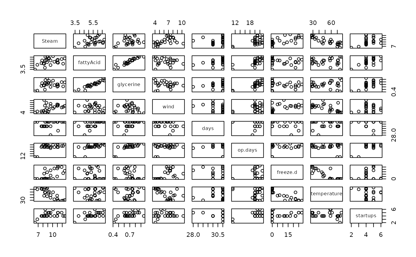
plot(steamUse)
 summary(fm1 <- lmrob(Steam ~ temperature + op.days, data=steamUse))
#>
#> Call:
#> lmrob(formula = Steam ~ temperature + op.days, data = steamUse)
#> \--> method = "MM"
#> Residuals:
#> Min 1Q Median 3Q Max
#> -1.2968 -0.2180 0.1365 0.4614 3.8812
#>
#> Coefficients:
#> Estimate Std. Error t value Pr(>|t|)
#> (Intercept) 3.087049 1.419653 2.175 0.0407 *
#> temperature -0.082858 0.006305 -13.142 6.80e-12 ***
#> op.days 0.514717 0.071214 7.228 3.05e-07 ***
#> ---
#> Signif. codes: 0 ‘***’ 0.001 ‘**’ 0.01 ‘*’ 0.05 ‘.’ 0.1 ‘ ’ 1
#>
#> Robust residual standard error: 0.5841
#> Multiple R-squared: 0.8696, Adjusted R-squared: 0.8577
#> Convergence in 9 IRWLS iterations
#>
#> Robustness weights:
#> 2 observations c(7,19) are outliers with |weight| = 0 ( < 0.004);
#> one weight is ~= 1. The remaining 22 ones are summarized as
#> Min. 1st Qu. Median Mean 3rd Qu. Max.
#> 0.6013 0.9133 0.9772 0.9313 0.9881 0.9987
#> Algorithmic parameters:
#> tuning.chi bb tuning.psi refine.tol
#> 1.548e+00 5.000e-01 4.685e+00 1.000e-07
#> rel.tol scale.tol solve.tol zero.tol
#> 1.000e-07 1.000e-10 1.000e-07 1.000e-10
#> eps.outlier eps.x warn.limit.reject warn.limit.meanrw
#> 4.000e-03 1.395e-10 5.000e-01 5.000e-01
#> nResample max.it best.r.s k.fast.s k.max
#> 500 50 2 1 200
#> maxit.scale trace.lev mts compute.rd fast.s.large.n
#> 200 0 1000 0 2000
#> psi subsampling cov
#> "bisquare" "nonsingular" ".vcov.avar1"
#> compute.outlier.stats
#> "SM"
#> seed : int(0)
## diagnoses 2 outliers: month of July, maybe company-wide summer vacations
## KS2014 alone seems not robust enough:
summary(fm.14 <- lmrob(Steam ~ temperature + op.days, data=steamUse,
setting="KS2014"))
#>
#> Call:
#> lmrob(formula = Steam ~ temperature + op.days, data = steamUse, setting = "KS2014")
#> \--> method = "SMDM"
#> Residuals:
#> Min 1Q Median 3Q Max
#> -1.62052 -0.46568 0.09035 0.47131 0.90895
#>
#> Coefficients:
#> Estimate Std. Error t value Pr(>|t|)
#> (Intercept) 9.243976 1.104246 8.371 2.76e-08 ***
#> temperature -0.073052 0.008028 -9.099 6.53e-09 ***
#> op.days 0.200307 0.045753 4.378 0.00024 ***
#> ---
#> Signif. codes: 0 ‘***’ 0.001 ‘**’ 0.01 ‘*’ 0.05 ‘.’ 0.1 ‘ ’ 1
#>
#> Robust residual standard error: 0.6705
#> Multiple R-squared: 0.8499, Adjusted R-squared: 0.8363
#> Convergence in 6 IRWLS iterations
#>
#> Robustness weights:
#> 19 weights are ~= 1. The remaining 6 ones are
#> 3 11 12 17 22 23
#> 0.9477 0.5665 0.9671 0.9875 0.9938 0.8497
#> Algorithmic parameters:
#> tuning.chi1 tuning.chi2 tuning.chi3 tuning.chi4
#> -5.000e-01 1.500e+00 NA 5.000e-01
#> bb tuning.psi1 tuning.psi2 tuning.psi3
#> 5.000e-01 -5.000e-01 1.500e+00 9.500e-01
#> tuning.psi4 refine.tol rel.tol scale.tol
#> NA 1.000e-07 1.000e-07 1.000e-10
#> solve.tol zero.tol eps.outlier eps.x
#> 1.000e-07 1.000e-10 4.000e-03 1.395e-10
#> warn.limit.reject warn.limit.meanrw
#> 5.000e-01 5.000e-01
#> nResample max.it best.r.s k.fast.s k.max
#> 1000 500 20 2 2000
#> maxit.scale trace.lev mts compute.rd numpoints
#> 200 0 1000 0 10
#> fast.s.large.n
#> 2000
#> setting psi subsampling
#> "KS2014" "lqq" "nonsingular"
#> cov compute.outlier.stats
#> ".vcov.w" "SMDM"
#> seed : int(0)
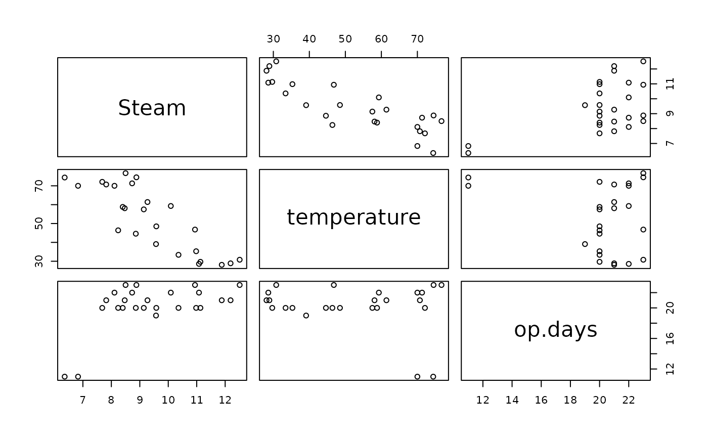
pairs(Steam ~ temperature+op.days, steamUse)
summary(fm1 <- lmrob(Steam ~ temperature + op.days, data=steamUse))
#>
#> Call:
#> lmrob(formula = Steam ~ temperature + op.days, data = steamUse)
#> \--> method = "MM"
#> Residuals:
#> Min 1Q Median 3Q Max
#> -1.2968 -0.2180 0.1365 0.4614 3.8812
#>
#> Coefficients:
#> Estimate Std. Error t value Pr(>|t|)
#> (Intercept) 3.087049 1.419653 2.175 0.0407 *
#> temperature -0.082858 0.006305 -13.142 6.80e-12 ***
#> op.days 0.514717 0.071214 7.228 3.05e-07 ***
#> ---
#> Signif. codes: 0 ‘***’ 0.001 ‘**’ 0.01 ‘*’ 0.05 ‘.’ 0.1 ‘ ’ 1
#>
#> Robust residual standard error: 0.5841
#> Multiple R-squared: 0.8696, Adjusted R-squared: 0.8577
#> Convergence in 9 IRWLS iterations
#>
#> Robustness weights:
#> 2 observations c(7,19) are outliers with |weight| = 0 ( < 0.004);
#> one weight is ~= 1. The remaining 22 ones are summarized as
#> Min. 1st Qu. Median Mean 3rd Qu. Max.
#> 0.6013 0.9133 0.9772 0.9313 0.9881 0.9987
#> Algorithmic parameters:
#> tuning.chi bb tuning.psi refine.tol
#> 1.548e+00 5.000e-01 4.685e+00 1.000e-07
#> rel.tol scale.tol solve.tol zero.tol
#> 1.000e-07 1.000e-10 1.000e-07 1.000e-10
#> eps.outlier eps.x warn.limit.reject warn.limit.meanrw
#> 4.000e-03 1.395e-10 5.000e-01 5.000e-01
#> nResample max.it best.r.s k.fast.s k.max
#> 500 50 2 1 200
#> maxit.scale trace.lev mts compute.rd fast.s.large.n
#> 200 0 1000 0 2000
#> psi subsampling cov
#> "bisquare" "nonsingular" ".vcov.avar1"
#> compute.outlier.stats
#> "SM"
#> seed : int(0)
## diagnoses 2 outliers: month of July, maybe company-wide summer vacations
## KS2014 alone seems not robust enough:
summary(fm.14 <- lmrob(Steam ~ temperature + op.days, data=steamUse,
setting="KS2014"))
#>
#> Call:
#> lmrob(formula = Steam ~ temperature + op.days, data = steamUse, setting = "KS2014")
#> \--> method = "SMDM"
#> Residuals:
#> Min 1Q Median 3Q Max
#> -1.62052 -0.46568 0.09035 0.47131 0.90895
#>
#> Coefficients:
#> Estimate Std. Error t value Pr(>|t|)
#> (Intercept) 9.243976 1.104246 8.371 2.76e-08 ***
#> temperature -0.073052 0.008028 -9.099 6.53e-09 ***
#> op.days 0.200307 0.045753 4.378 0.00024 ***
#> ---
#> Signif. codes: 0 ‘***’ 0.001 ‘**’ 0.01 ‘*’ 0.05 ‘.’ 0.1 ‘ ’ 1
#>
#> Robust residual standard error: 0.6705
#> Multiple R-squared: 0.8499, Adjusted R-squared: 0.8363
#> Convergence in 6 IRWLS iterations
#>
#> Robustness weights:
#> 19 weights are ~= 1. The remaining 6 ones are
#> 3 11 12 17 22 23
#> 0.9477 0.5665 0.9671 0.9875 0.9938 0.8497
#> Algorithmic parameters:
#> tuning.chi1 tuning.chi2 tuning.chi3 tuning.chi4
#> -5.000e-01 1.500e+00 NA 5.000e-01
#> bb tuning.psi1 tuning.psi2 tuning.psi3
#> 5.000e-01 -5.000e-01 1.500e+00 9.500e-01
#> tuning.psi4 refine.tol rel.tol scale.tol
#> NA 1.000e-07 1.000e-07 1.000e-10
#> solve.tol zero.tol eps.outlier eps.x
#> 1.000e-07 1.000e-10 4.000e-03 1.395e-10
#> warn.limit.reject warn.limit.meanrw
#> 5.000e-01 5.000e-01
#> nResample max.it best.r.s k.fast.s k.max
#> 1000 500 20 2 2000
#> maxit.scale trace.lev mts compute.rd numpoints
#> 200 0 1000 0 10
#> fast.s.large.n
#> 2000
#> setting psi subsampling
#> "KS2014" "lqq" "nonsingular"
#> cov compute.outlier.stats
#> ".vcov.w" "SMDM"
#> seed : int(0)
pairs(Steam ~ temperature+op.days, steamUse)