Extreme Data examples
xtrData.Rdx30o50, called ‘'XX'’ in the thesis, has been a running
case for which mc() had failed to converge.
A numeric vector of 50 values, 30 of which are very close to zero,
specifically, their absolute values are less than 1.5e-15.
The remaining 20 values (11 negative, 9 positive) have absolute values between 0.0022 and 1.66.
data(x30o50, package="robustbase")Format
A summary is
    Min.  1st Qu.   Median     Mean  3rd Qu.     Max.
-1.66006  0.00000  0.00000 -0.04155  0.00000  1.29768
notably the 1st to 3rd quartiles are all very close to zero.
Details
a good robust method will treat the 60% “almost zero” values as “good” data and all other as outliers.
This is somewhat counter intuitive to typical human perception where the 30 almost-zero numbers would be considered as inliers and the remaining 20 as “good” data.
The original mc() algorithm and also the amendments up to 2022
(robustbase versions before 0.95) would fail to converge unless (in
newer versions) eps1 was increased, e.g., only by a factor of 10,
to eps1 = 1e-13.
References
Lukas Graz (2021); unpublished BSc thesis, see mc.
Examples
data(x30o50)
## have 4 duplicated values :
table(dX <- duplicated(x30o50))
#>
#> FALSE TRUE
#> 46 4
x30o50[dX] # 0 2.77e-17 4.16e-17 2.08e-16
#> [1] 2.081668e-16 0.000000e+00 4.163336e-17 2.775558e-17
sort(x30o50[dX]) * 2^56 # 0 2 3 15
#> [1] 0 2 3 15
## and they are c(0,2,3,15)*2^-56
table(sml <- abs(x30o50) < 1e-11)# 20 30
#>
#> FALSE TRUE
#> 20 30
summary(x30o50[ sml]) # -1.082e-15 ... 1.499e-15 ; mean = 9.2e-19 ~~ 0
#> Min. 1st Qu. Median Mean 3rd Qu. Max.
#> -1.082e-15 -1.631e-16 1.388e-17 9.252e-19 2.012e-16 1.499e-15
summary(x30o50[!sml])
#> Min. 1st Qu. Median Mean 3rd Qu. Max.
#> -1.6601 -0.4689 -0.0550 -0.1039 0.3986 1.2977
## Min. 1st Qu. Median Mean 3rd Qu. Max.
## -1.6601 -0.4689 -0.0550 -0.1039 0.3986 1.2977
op <- par(mfrow=c(3,1), mgp=c(1.5, .6, 0), mar = .3+c(2,3:1))
(Fn. <- ecdf(x30o50)) # <- only 46 knots (as have 4 duplications)
#> Empirical CDF
#> Call: ecdf(x30o50)
#> x[1:46] = -1.6601, -1.1635, -1.0963, ..., 0.88786, 1.2977
plot(Fn.) ## and zoom in (*drastically*) to around x=0 :
for(f in c(1e-13, 1.5e-15)) {
plot(Fn., xval=f*seq(-1,1, length.out = 1001), ylim=c(0,1), main="[zoomed in]")
if(f == 1e-13) rect(-1e-15,0, +1e-15, 1, col="thistle", border=1)
plot(Fn., add=TRUE)
}
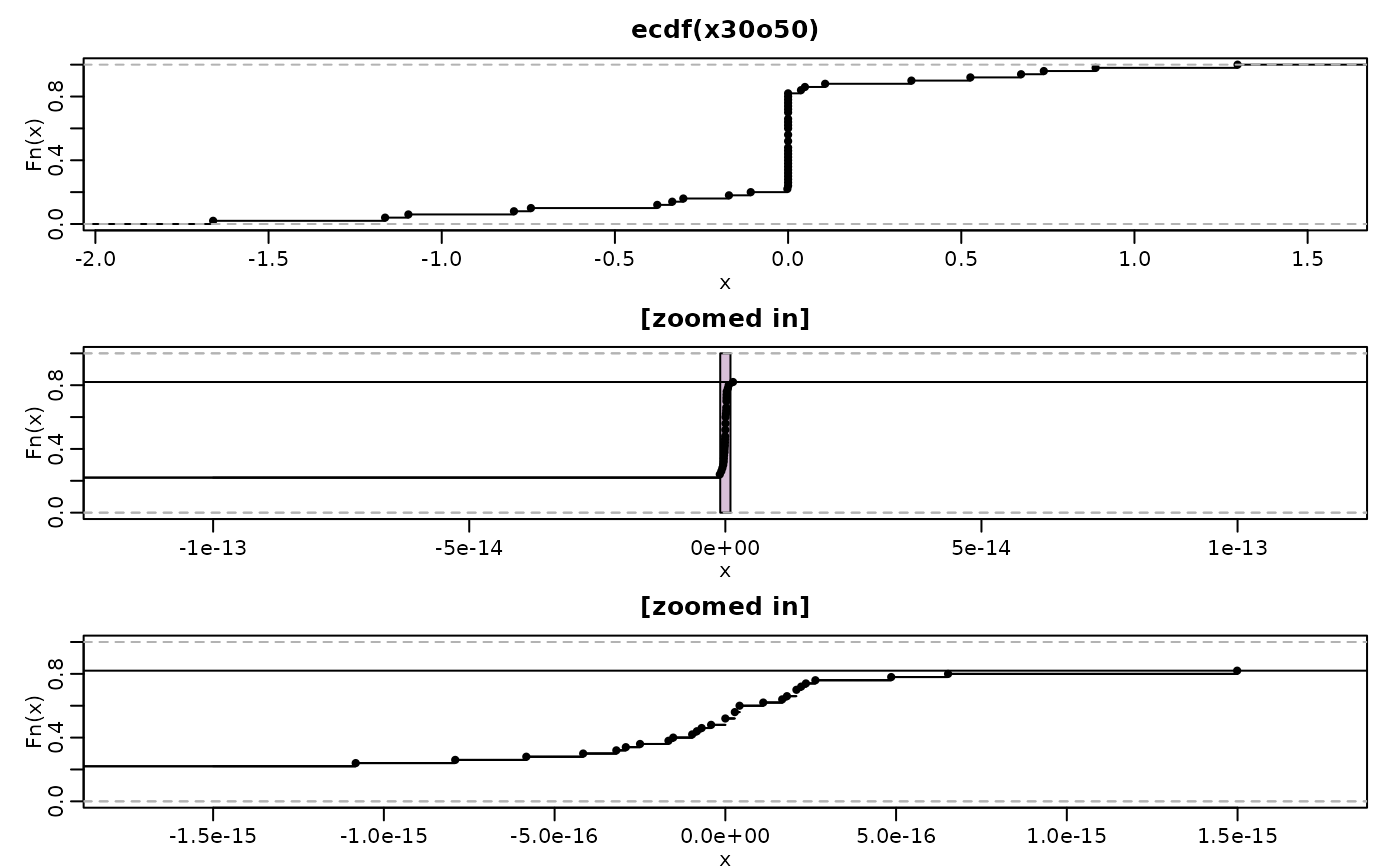 par(op)
mcOld <- function(x, ..., doScale=TRUE) mc(x, doScale=doScale, c.huberize=Inf, ...)
try( mcOld(x30o50) ) # Error: .. not 'converged' in 100 iteration
#> Warning: maximal number of iterations (100 =? 100) reached prematurely
#> Error in mc(x, doScale = doScale, c.huberize = Inf, ...) :
#> mc(): not 'converged' in 100 iterations; try enlarging eps1, eps2 !?
#>
mcOld(x30o50, eps1 = 1e-12) # -0.152
#> [1] -0.1523899
(mcX <- mc(x30o50)) # -7.10849e-13
#> [1] -7.10849e-13
stopifnot(exprs = {
all.equal(-7.10848988e-13, mcX, tol = 1e-9)
all.equal(mcX, mc(1e30*x30o50), tol = 4e-4) # not so close
})
table(sml <- abs(x30o50) < 1e-8)# 20 30
#>
#> FALSE TRUE
#> 20 30
range(x30o50[sml])
#> [1] -1.082467e-15 1.498801e-15
x0o50 <- x30o50; x0o50[sml] <- 0
(mcX0 <- mc(x0o50))
#> [1] -0.3784454
stopifnot(exprs = {
all.equal(-0.378445401788, mcX0, tol=1e-12)
all.equal(-0.099275805349, mc(x30o50[!sml]) -> mcL, tol=2e-11)
all.equal(mcL, mcOld(x30o50[!sml]))
})
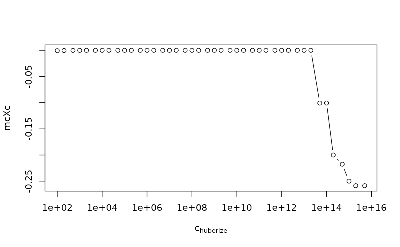
## -- some instability also wrt c.huberize:
mcHubc <- function(dat, ...)
function(cc) vapply(cc, function(c) mc(dat, c.huberize = c, ...), -1.)
mcH50 <- mcHubc(x30o50)
head(cHs <- c(sort(outer(c(1, 2, 5), 10^(2:15))), Inf), 9)
#> [1] 100 200 500 1000 2000 5000 10000 20000 50000
mcXc <- mcH50(cHs)
plot( mcXc ~ cHs, type="b", log="x" , xlab=quote(c[huberize]))
par(op)
mcOld <- function(x, ..., doScale=TRUE) mc(x, doScale=doScale, c.huberize=Inf, ...)
try( mcOld(x30o50) ) # Error: .. not 'converged' in 100 iteration
#> Warning: maximal number of iterations (100 =? 100) reached prematurely
#> Error in mc(x, doScale = doScale, c.huberize = Inf, ...) :
#> mc(): not 'converged' in 100 iterations; try enlarging eps1, eps2 !?
#>
mcOld(x30o50, eps1 = 1e-12) # -0.152
#> [1] -0.1523899
(mcX <- mc(x30o50)) # -7.10849e-13
#> [1] -7.10849e-13
stopifnot(exprs = {
all.equal(-7.10848988e-13, mcX, tol = 1e-9)
all.equal(mcX, mc(1e30*x30o50), tol = 4e-4) # not so close
})
table(sml <- abs(x30o50) < 1e-8)# 20 30
#>
#> FALSE TRUE
#> 20 30
range(x30o50[sml])
#> [1] -1.082467e-15 1.498801e-15
x0o50 <- x30o50; x0o50[sml] <- 0
(mcX0 <- mc(x0o50))
#> [1] -0.3784454
stopifnot(exprs = {
all.equal(-0.378445401788, mcX0, tol=1e-12)
all.equal(-0.099275805349, mc(x30o50[!sml]) -> mcL, tol=2e-11)
all.equal(mcL, mcOld(x30o50[!sml]))
})
## -- some instability also wrt c.huberize:
mcHubc <- function(dat, ...)
function(cc) vapply(cc, function(c) mc(dat, c.huberize = c, ...), -1.)
mcH50 <- mcHubc(x30o50)
head(cHs <- c(sort(outer(c(1, 2, 5), 10^(2:15))), Inf), 9)
#> [1] 100 200 500 1000 2000 5000 10000 20000 50000
mcXc <- mcH50(cHs)
plot( mcXc ~ cHs, type="b", log="x" , xlab=quote(c[huberize]))
 plot((-mcXc) ~ cHs, type="b", log="xy", xlab=quote(c[huberize]))
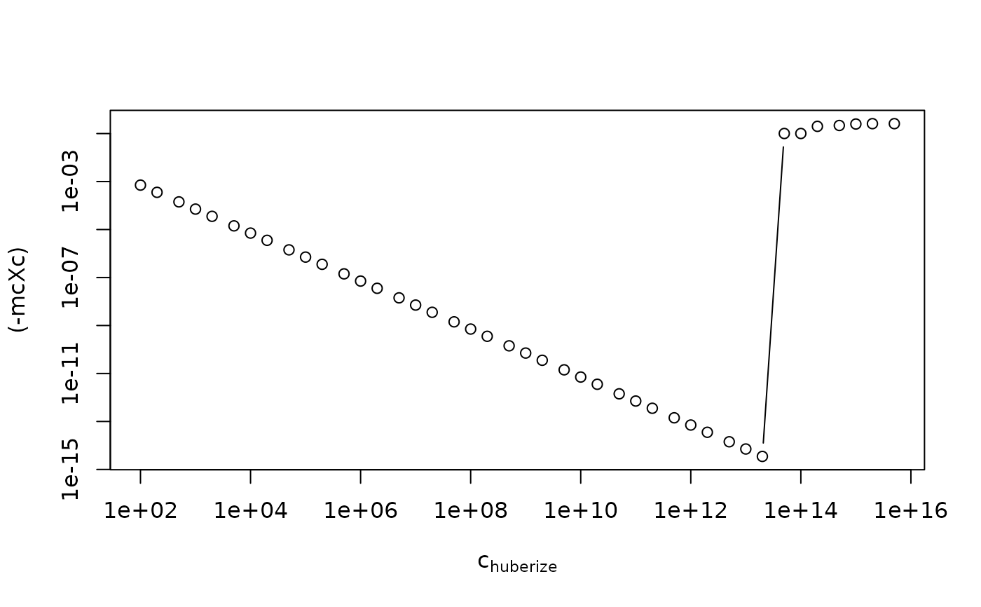 ## but for "regular" outlier skew data, there's no such dependency:
mcXcu <- mcHubc(cushny)(cHs)
stopifnot( abs(mcXcu - mcXcu[1]) < 1e-15)
## but for "regular" outlier skew data, there's no such dependency:
mcXcu <- mcHubc(cushny)(cHs)
stopifnot( abs(mcXcu - mcXcu[1]) < 1e-15)