Provide a tibble-friendly framework to visualize a correlation
matrix. Wrapper around the R base function
corrplot(). Compared to
corrplot(), it can handle directly the output of the
functions cor_mat() (in rstatix), rcorr() (in Hmisc),
correlate() (in corrr) and cor() (in stats).
The p-values contained in the outputs of the functions
cor_mat() and rcorr() are automatically detected and
used in the visualization.
Arguments
- cor.mat
the correlation matrix to visualize
- method
Character, the visualization method of correlation matrix to be used. Currently, it supports seven methods, named
'circle'(default),'square','ellipse','number','pie','shade'and'color'. See examples for details.The areas of circles or squares show the absolute value of corresponding correlation coefficients. Method
'pie'and'shade'came from Michael Friendly's job (with some adjustment about the shade added on), and'ellipse'came from D.J. Murdoch and E.D. Chow's job, see in section References.- type
Character,
'full'(default),'upper'or'lower', display full matrix, lower triangular or upper triangular matrix.- palette
character vector containing the color palette.
- p.mat
matrix of p-value corresponding to the correlation matrix.
- significant.level
significant level, if the p-value is bigger than
significant.level, then the corresponding correlation coefficient is regarded as insignificant.- insignificant
character, specialized insignificant correlation coefficients, "cross" (default), "blank". If "blank", wipe away the corresponding glyphs; if "cross", add crosses (X) on corresponding glyphs.
- label
logical value. If TRUE, shows the correlation coefficient labels.
- font.label
a list with one or more of the following elements: size (e.g., 1), color (e.g., "black") and style (e.g., "bold"). Used to customize the correlation coefficient labels. For example
font.label = list(size = 1, color = "black", style = "bold").- ...
additional options not listed (i.e. "tl.cex") here to pass to corrplot.
Examples
# Compute correlation matrix
#::::::::::::::::::::::::::::::::::::::::::
cor.mat <- mtcars %>%
select(mpg, disp, hp, drat, wt, qsec) %>%
cor_mat()
# Visualize correlation matrix
#::::::::::::::::::::::::::::::::::::::::::
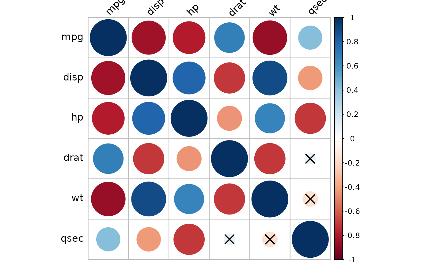
# Full correlation matrix,
# insignificant correlations are marked by crosses
cor.mat %>% cor_plot()
 # Reorder by correlation coefficient
# pull lower triangle and visualize
cor.lower.tri <- cor.mat %>%
cor_reorder() %>%
pull_lower_triangle()
cor.lower.tri %>% cor_plot()
# Reorder by correlation coefficient
# pull lower triangle and visualize
cor.lower.tri <- cor.mat %>%
cor_reorder() %>%
pull_lower_triangle()
cor.lower.tri %>% cor_plot()
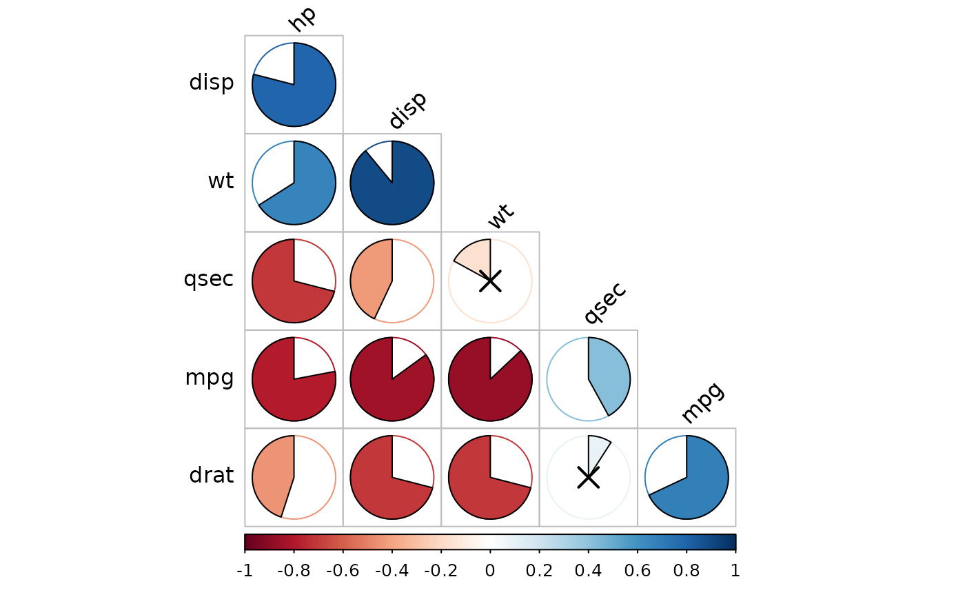
 # Change visualization methods
#::::::::::::::::::::::::::::::::::::::::::
cor.lower.tri %>%
cor_plot(method = "pie")
# Change visualization methods
#::::::::::::::::::::::::::::::::::::::::::
cor.lower.tri %>%
cor_plot(method = "pie")
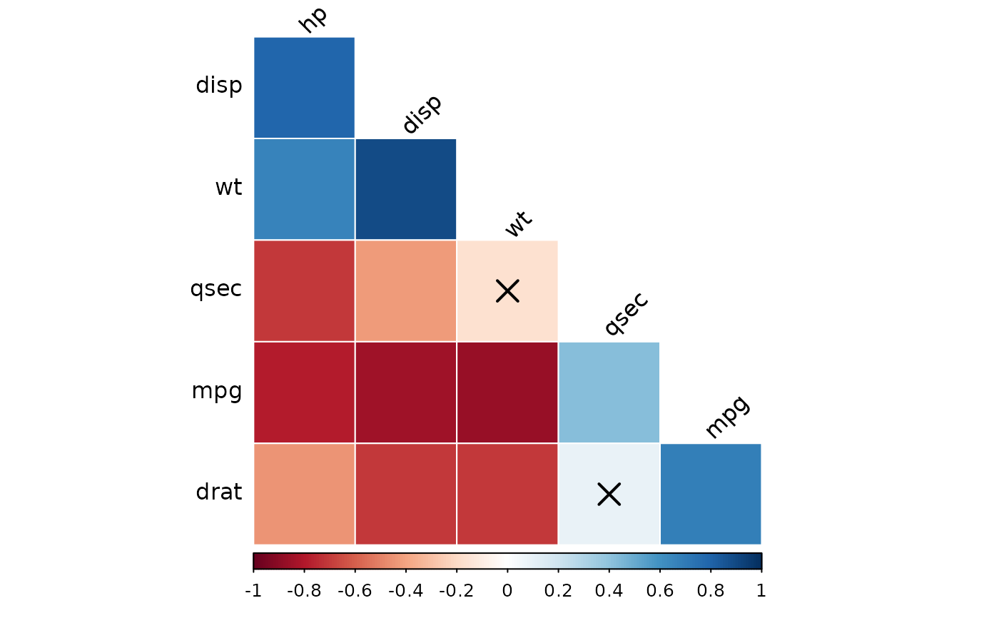
 cor.lower.tri %>%
cor_plot(method = "color")
cor.lower.tri %>%
cor_plot(method = "color")
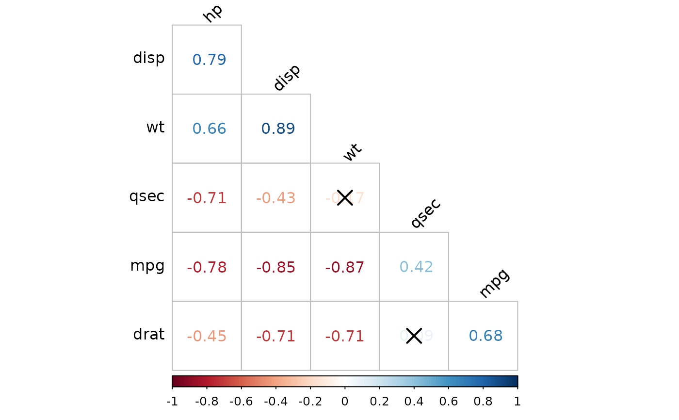
 cor.lower.tri %>%
cor_plot(method = "number")
cor.lower.tri %>%
cor_plot(method = "number")
 # Show the correlation coefficient: label = TRUE
# Blank the insignificant correlation
#::::::::::::::::::::::::::::::::::::::::::
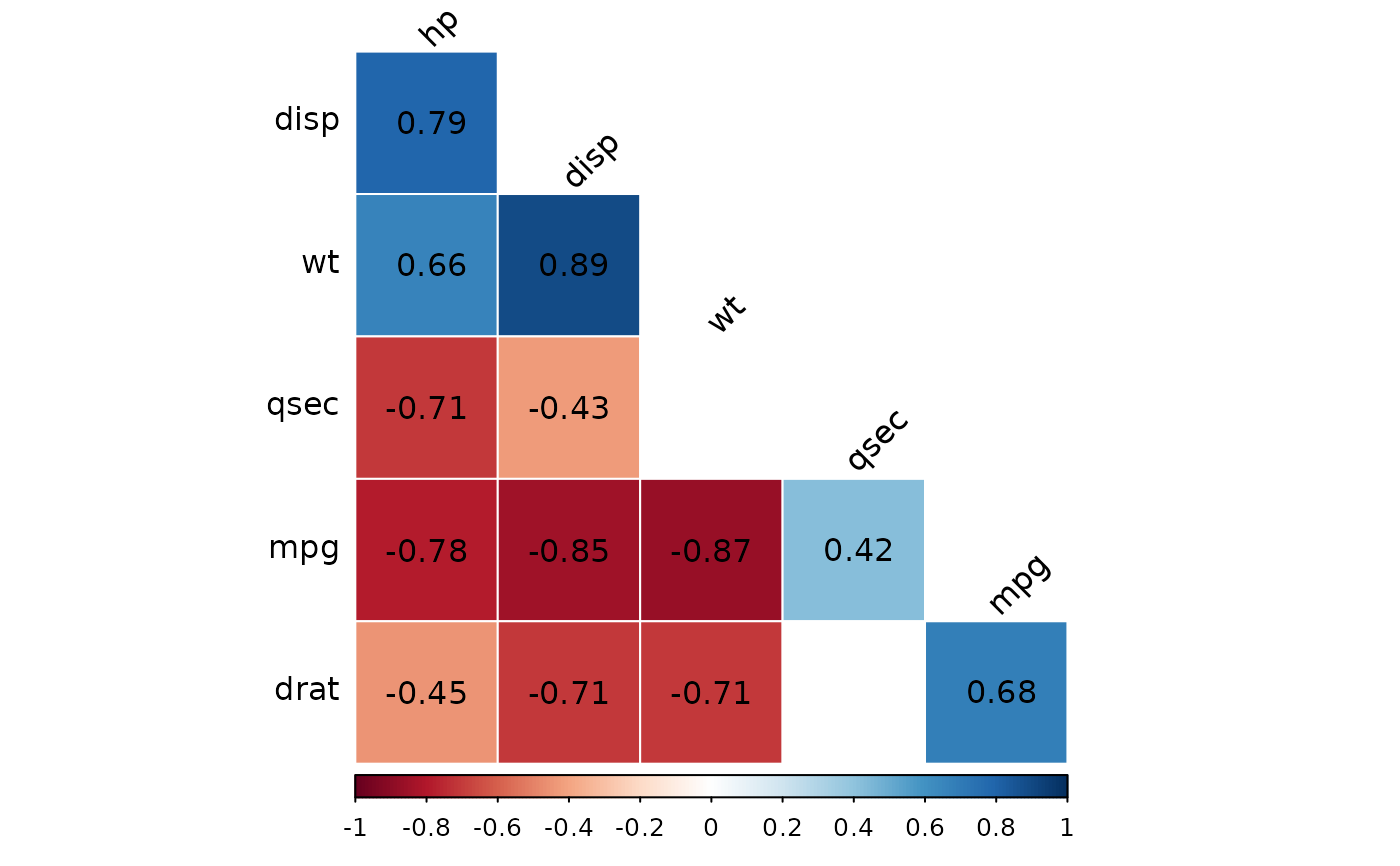
cor.lower.tri %>%
cor_plot(
method = "color",
label = TRUE,
insignificant = "blank"
)
# Show the correlation coefficient: label = TRUE
# Blank the insignificant correlation
#::::::::::::::::::::::::::::::::::::::::::
cor.lower.tri %>%
cor_plot(
method = "color",
label = TRUE,
insignificant = "blank"
)
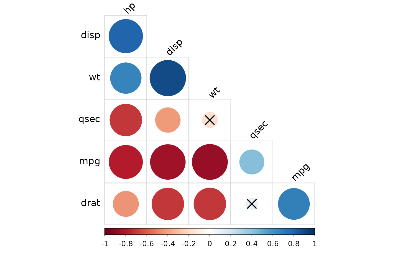
 # Change the color palettes
#::::::::::::::::::::::::::::::::::::::::::
# Using custom color palette
# Require ggpubr: install.packages("ggpubr")
if(require("ggpubr")){
my.palette <- get_palette(c("red", "white", "blue"), 200)
cor.lower.tri %>%
cor_plot(palette = my.palette)
}
#> Loading required package: ggpubr
#> Loading required package: ggplot2
# Change the color palettes
#::::::::::::::::::::::::::::::::::::::::::
# Using custom color palette
# Require ggpubr: install.packages("ggpubr")
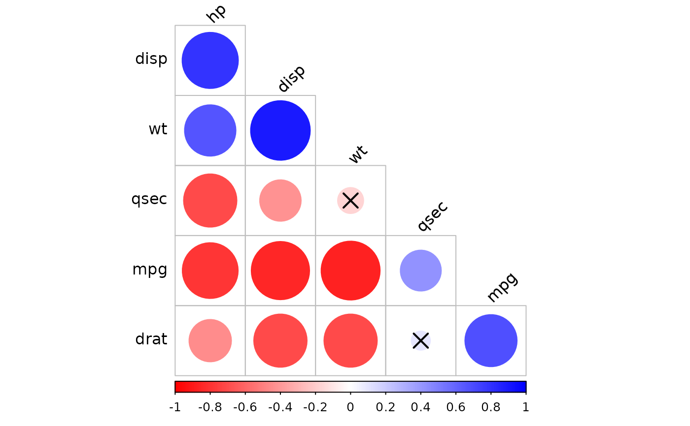
if(require("ggpubr")){
my.palette <- get_palette(c("red", "white", "blue"), 200)
cor.lower.tri %>%
cor_plot(palette = my.palette)
}
#> Loading required package: ggpubr
#> Loading required package: ggplot2
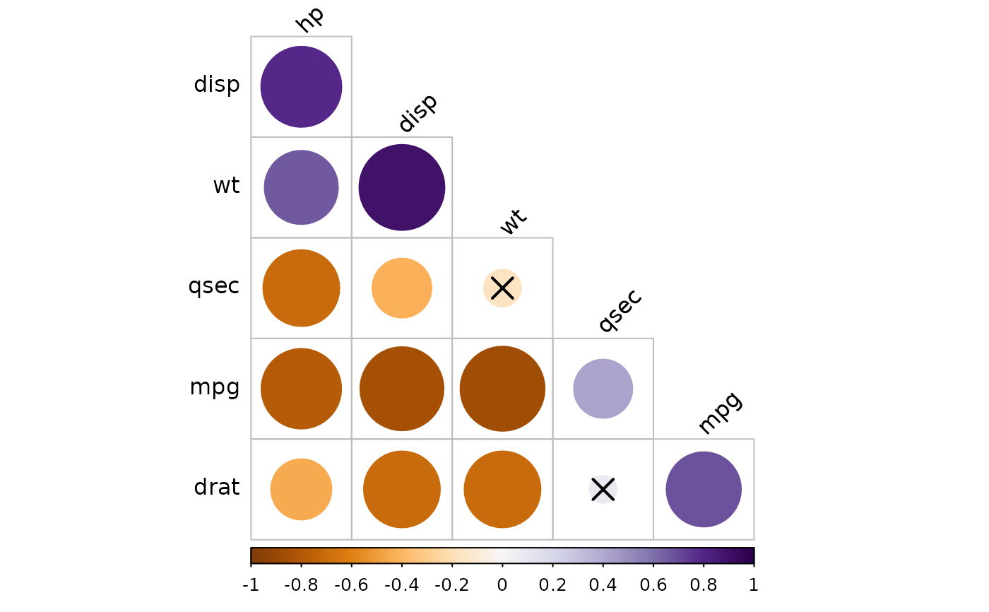
 # Using RcolorBrewer color palette
if(require("ggpubr")){
my.palette <- get_palette("PuOr", 200)
cor.lower.tri %>%
cor_plot(palette = my.palette)
}
# Using RcolorBrewer color palette
if(require("ggpubr")){
my.palette <- get_palette("PuOr", 200)
cor.lower.tri %>%
cor_plot(palette = my.palette)
}