rxode2 Event Types

rxode2 event tables

In general, rxode2 event tables follow NONMEM dataset convention with the exceptions:

The compartment data item (cmt) can be a string/factor with compartment names
- You may turn off a compartment with a negative compartment number or “-cmt” where cmt is the compartment name.
- The compartment data item (cmt) can still be a number, the number of the compartment is defined by the appearance of the compartment name in the model. This can be tedious to count, so you can specify compartment numbers easier by using the cmt(cmtName) at the beginning of the model.
An additional column, dur can specify the duration of infusions;
- Bioavailability changes will change the rate of infusion since dur/amt are fixed in the input data.
- Similarly, when specifying rate/amt for an infusion, the bioavailability will change the infusion duration since rate/amt are fixed in the input data.
Some infrequent NONMEM columns are not supported: pcmt, call.
NONMEM-style events are supported (0: Observation, 1: Dose, 2: Other, 3: Reset, 4: Reset+Dose). Additional events are supported:
- evid=5 or replace event; This replaces the value of a compartment with the value specified in the amt column. This is equivalent to deSolve=replace.
- evid=6 or multiply event; This multiplies the value in the compartment with the value specified by the amt column. This is equivalent to deSolve=multiply.
- evid=7 or transit compartment model/phantom event. This puts the dose in the dose() function and calculates time since last dose tad() but doesn’t actually put the dose in the compartment. This allows the transit() function to easily apply to the compartment.

Here are the legal entries to a data table:

Data Item	Meaning	Notes
id	Individual identifier	Can be a integer, factor, character, or numeric
time	Individual time	Numeric for each time.
amt	dose amount	Positive for doses zero/NA for observations
rate	infusion rate	When specified the infusion duration will be dur=amt/rate
		rate = -1, rate modeled; rate = -2, duration modeled
dur	infusion duration	When specified the infusion rate will be rate = amt/dur
evid	event ID	0=Observation; 1=Dose; 2=Other; 3=Reset; 4=Reset+Dose; 5=Replace; 6=Multiply;7=Transit
cmt	Compartment	Represents compartment #/name for dose/observation
ss	Steady State Flag	0 = non-steady-state; 1=steady state; 2=steady state +prior states
ii	Inter-dose Interval	Time between doses.
addl	# of additional doses	Number of doses like the current dose.

Other notes:

The evid can be the classic RxODE (described here) or the NONMEM-style evid described above.
NONMEM’s DV is not required; rxode2 is a ODE solving framework.
NONMEM’s MDV is not required, since it is captured in EVID.
Instead of NONMEM-compatible data, it can accept deSolve compatible data-frames.

When returning the rxode2 solved data-set there are a few additional event ids (EVID) that you may see depending on the solving options:

EVID = -1 is when a modeled rate ends (corresponds to rate = -1)
EVID = -2 is when a modeled duration ends (corresponds to rate=-2)
EVID = -10 when a rate specified zero-order infusion ends (corresponds to rate > 0)
EVID = -20 when a duration specified zero-order infusion ends (corresponds to dur > 0)
EVID = 101, 102, 103,... These correspond to the 1, 2, 3, … modeled time (mtime).

These can only be accessed when solving with the option combination addDosing=TRUE and subsetNonmem=FALSE. If you want to see the classic EVID equivalents you can use addDosing=NA.

To illustrate the event types we will use the model from the original rxode2 tutorial.

library(rxode2)

#> rxode2 3.0.3 using 2 threads (see ?getRxThreads)
#>   no cache: create with `rxCreateCache()`

## Model from rxode2 tutorial

m1 <- function() {
  ini({
    KA   <- 2.94E-01
    CL   <- 1.86E+01
    V2   <- 4.02E+01
    Q    <- 1.05E+01
    V3   <- 2.97E+02
    Kin  <- 1
    Kout <- 1
    EC50 <- 200
    ## Added modeled bioavaiblity, duration and rate
    fdepot <- 1
    durDepot <- 8
    rateDepot <- 1250
  })
  model({
    C2 <- centr/V2
    C3 <- peri/V3
    d/dt(depot) <- -KA*depot
    f(depot) <- fdepot
    dur(depot) <- durDepot
    rate(depot) <- rateDepot
    d/dt(centr) <- KA*depot - CL*C2 - Q*C2 + Q*C3
    d/dt(peri)  <-                    Q*C2 - Q*C3
    d/dt(eff)  <- Kin - Kout*(1-C2/(EC50+C2))*eff
    eff(0) <- 1
  })
}

Bolus/Additive Doses

A bolus dose is the default type of dose in rxode2 and only requires the amt/dose. Note that this uses the convenience function et() described in the rxode2 event tables

ev <- et(timeUnits="hr") %>%
    et(amt=10000, ii=12,until=24) %>%
    et(seq(0, 24, length.out=100))

ev

#> -- EventTable with 101 records --
#> 1 dosing records (see x$get.dosing(); add with add.dosing or et)
#> 100 observation times (see x$get.sampling(); add with add.sampling or et)
#> multiple doses in `addl` columns, expand with x$expand(); or etExpand(x)
#> -- First part of x: --
#> # A tibble: 101 x 5
#>     time   amt  ii  addl evid         
#>      [h] <dbl> [h] <int> <evid>       
#>  1 0        NA  NA    NA 0:Observation
#>  2 0     10000  12     2 1:Dose (Add) 
#>  3 0.242    NA  NA    NA 0:Observation
#>  4 0.485    NA  NA    NA 0:Observation
#>  5 0.727    NA  NA    NA 0:Observation
#>  6 0.970    NA  NA    NA 0:Observation
#>  7 1.21     NA  NA    NA 0:Observation
#>  8 1.45     NA  NA    NA 0:Observation
#>  9 1.70     NA  NA    NA 0:Observation
#> 10 1.94     NA  NA    NA 0:Observation
#> # i 91 more rows

rxSolve(m1, ev) %>% plot(C2) +
    xlab("Time")

#> i parameter labels from comments are typically ignored in non-interactive mode

#> i Need to run with the source intact to parse comments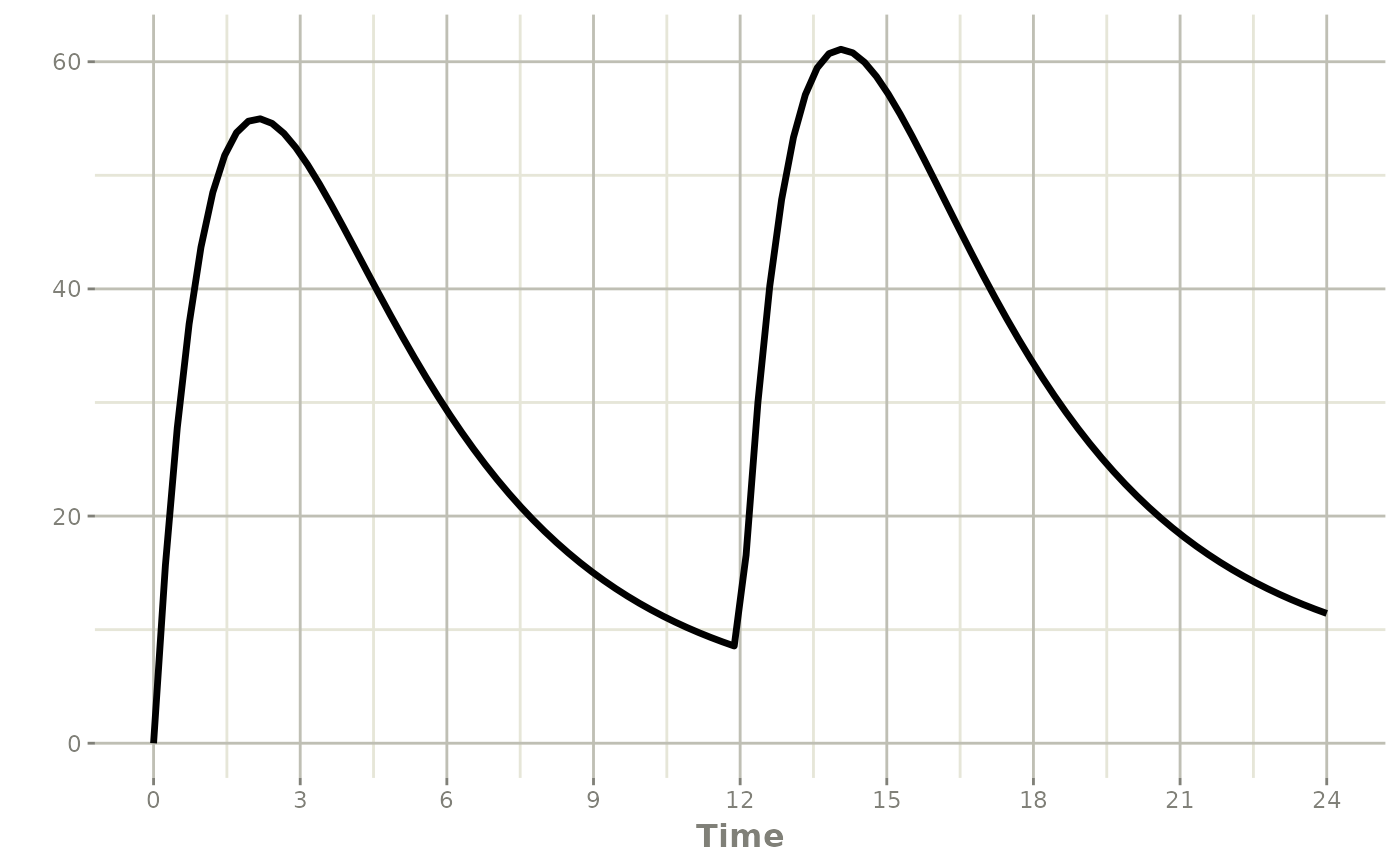

Infusion Doses

There are a few different type of infusions that rxode2 supports:

Constant Rate Infusion (rate)
Constant Duration Infusion (dur)
Estimated Rate of Infusion
Estimated Duration of Infusion

Constant Infusion (in terms of duration and rate)

The next type of event is an infusion; There are two ways to specify an infusion; The first is the dur keyword.

An example of this is:

ev <- et(timeUnits="hr") %>%
    et(amt=10000, ii=12,until=24, dur=8) %>%
    et(seq(0, 24, length.out=100))

ev

#> -- EventTable with 101 records --
#> 1 dosing records (see x$get.dosing(); add with add.dosing or et)
#> 100 observation times (see x$get.sampling(); add with add.sampling or et)
#> multiple doses in `addl` columns, expand with x$expand(); or etExpand(x)
#> -- First part of x: --
#> # A tibble: 101 x 6
#>     time   amt  ii  addl evid          dur
#>      [h] <dbl> [h] <int> <evid>        [h]
#>  1 0        NA  NA    NA 0:Observation  NA
#>  2 0     10000  12     2 1:Dose (Add)    8
#>  3 0.242    NA  NA    NA 0:Observation  NA
#>  4 0.485    NA  NA    NA 0:Observation  NA
#>  5 0.727    NA  NA    NA 0:Observation  NA
#>  6 0.970    NA  NA    NA 0:Observation  NA
#>  7 1.21     NA  NA    NA 0:Observation  NA
#>  8 1.45     NA  NA    NA 0:Observation  NA
#>  9 1.70     NA  NA    NA 0:Observation  NA
#> 10 1.94     NA  NA    NA 0:Observation  NA
#> # i 91 more rows

rxSolve(m1, ev) %>% plot(depot, C2) +
    xlab("Time")

#> i parameter labels from comments are typically ignored in non-interactive mode

#> i Need to run with the source intact to parse comments

It can be also specified by the rate component:

ev <- et(timeUnits="hr") %>%
    et(amt=10000, ii=12,until=24, rate=10000/8) %>%
    et(seq(0, 24, length.out=100))

ev

#> -- EventTable with 101 records --
#> 1 dosing records (see x$get.dosing(); add with add.dosing or et)
#> 100 observation times (see x$get.sampling(); add with add.sampling or et)
#> multiple doses in `addl` columns, expand with x$expand(); or etExpand(x)
#> -- First part of x: --
#> # A tibble: 101 x 6
#>     time   amt rate        ii  addl evid         
#>      [h] <dbl> <rate/dur> [h] <int> <evid>       
#>  1 0        NA NA          NA    NA 0:Observation
#>  2 0     10000  1250       12     2 1:Dose (Add) 
#>  3 0.242    NA NA          NA    NA 0:Observation
#>  4 0.485    NA NA          NA    NA 0:Observation
#>  5 0.727    NA NA          NA    NA 0:Observation
#>  6 0.970    NA NA          NA    NA 0:Observation
#>  7 1.21     NA NA          NA    NA 0:Observation
#>  8 1.45     NA NA          NA    NA 0:Observation
#>  9 1.70     NA NA          NA    NA 0:Observation
#> 10 1.94     NA NA          NA    NA 0:Observation
#> # i 91 more rows

rxSolve(m1, ev) %>% plot(depot, C2) +
    xlab("Time")

#> i parameter labels from comments are typically ignored in non-interactive mode

#> i Need to run with the source intact to parse comments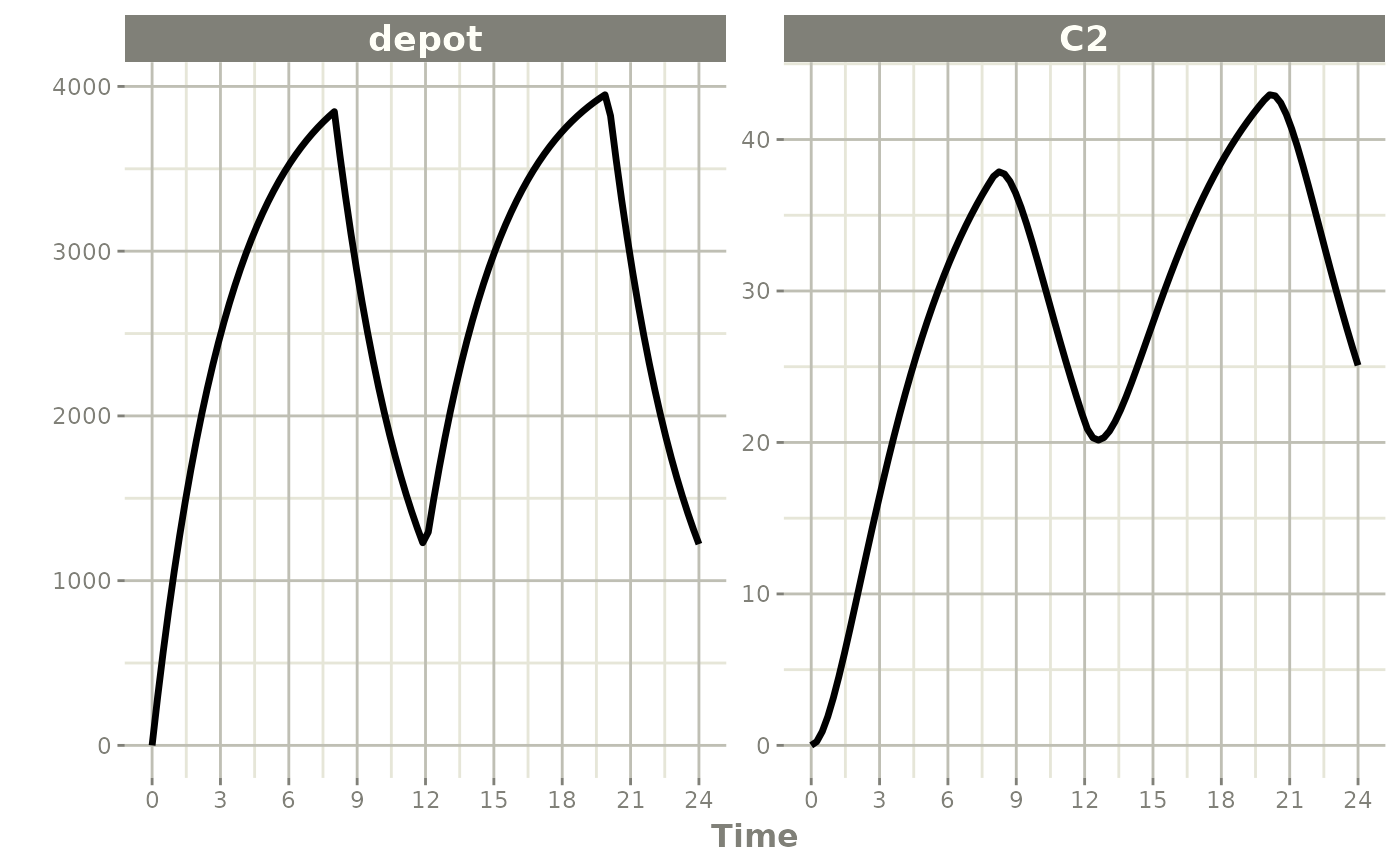

These are the same with the exception of how bioavailability changes the infusion.

In the case of modeling rate, a bioavailability decrease, decreases the infusion duration, as in NONMEM. For example:

rxSolve(m1, ev, c(fdepot=0.25)) %>% plot(depot, C2) +
    xlab("Time")

#> i parameter labels from comments are typically ignored in non-interactive mode

#> i Need to run with the source intact to parse comments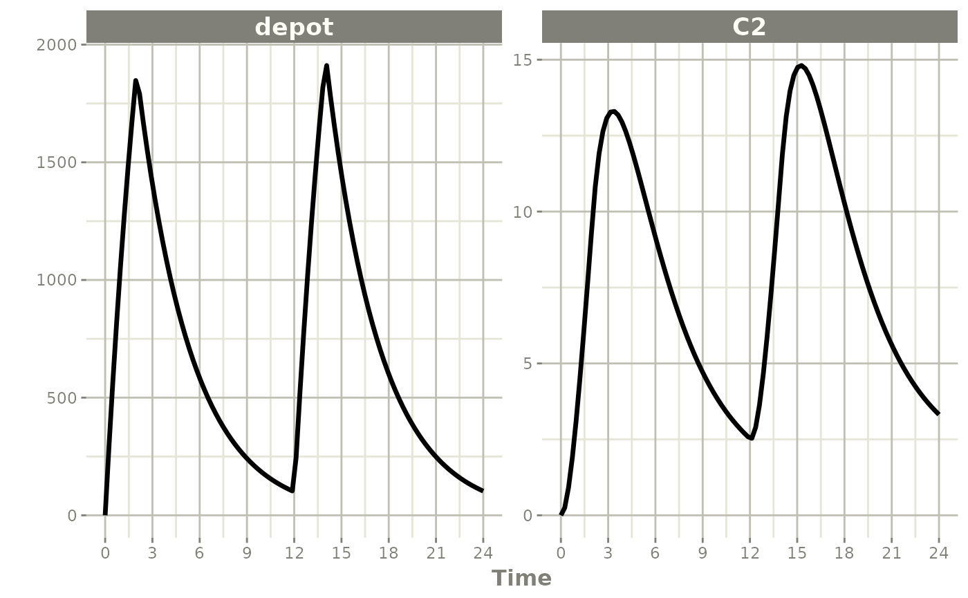

Similarly increasing the bioavailability increases the infusion duration.

rxSolve(m1, ev, c(fdepot=1.25)) %>% plot(depot, C2) +
    xlab("Time")

#> i parameter labels from comments are typically ignored in non-interactive mode

#> i Need to run with the source intact to parse comments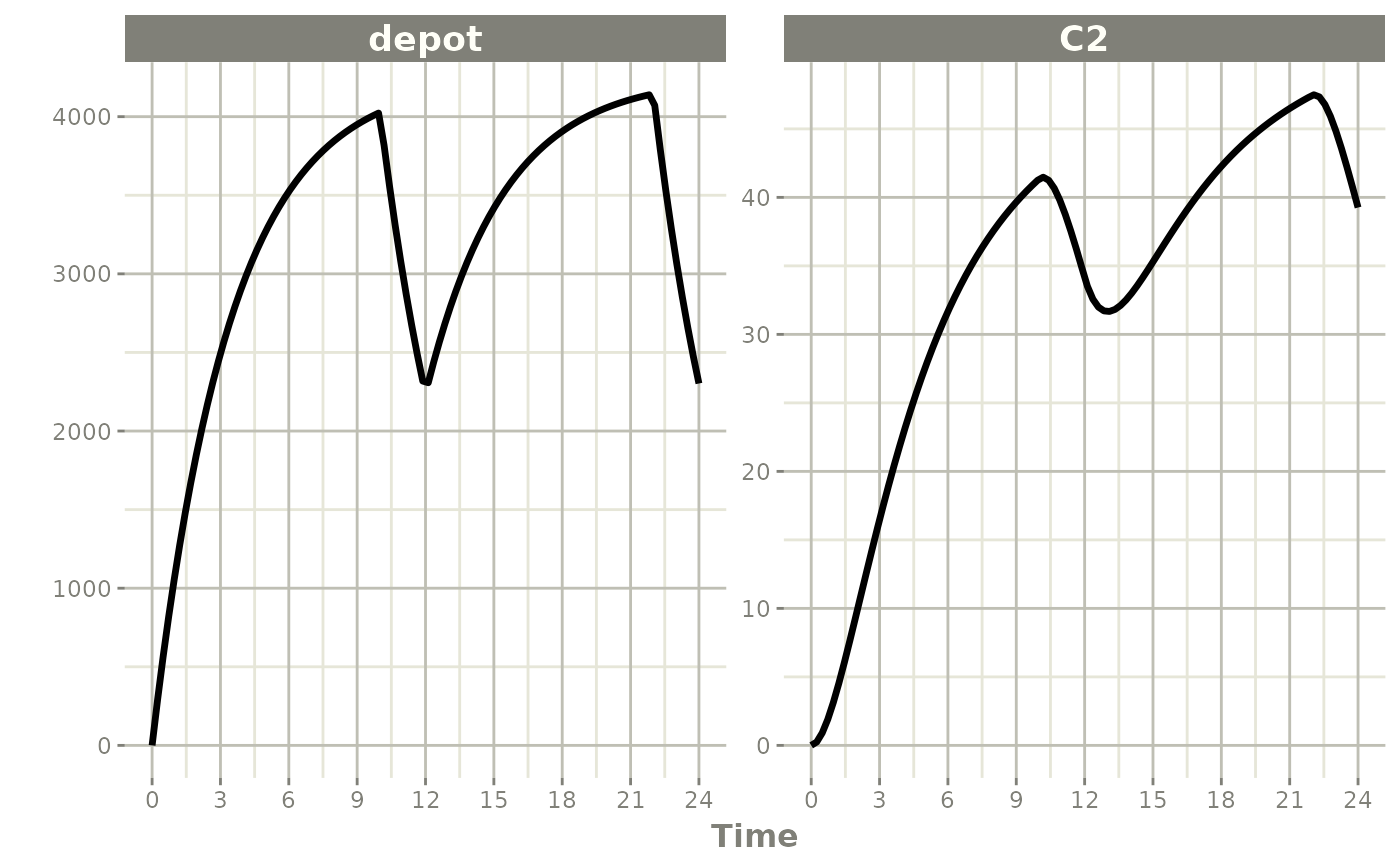

The rationale for this behavior is that the rate and amt are specified by the event table, so the only thing that can change with a bioavailability increase is the duration of the infusion.

If you specify the amt and dur components in the event table, bioavailability changes affect the rate of infusion.

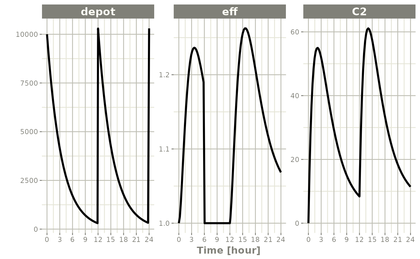
ev <- et(timeUnits="hr") %>%
    et(amt=10000, ii=12,until=24, dur=8) %>%
    et(seq(0, 24, length.out=100))

You can see the side-by-side comparison of bioavailability changes affecting rate instead of duration with these records in the following plots:

library(ggplot2)
library(patchwork)

p1 <- rxSolve(m1, ev, c(fdepot=1.25)) %>% plot(depot) +
    xlab("Time") + ylim(0,5000)

#> i parameter labels from comments are typically ignored in non-interactive mode

#> i Need to run with the source intact to parse comments

p2 <- rxSolve(m1, ev, c(fdepot=0.25)) %>% plot(depot) +
    xlab("Time")+ ylim(0,5000)

#> i parameter labels from comments are typically ignored in non-interactive mode
#> i Need to run with the source intact to parse comments

## Use patchwork syntax to combine plots
p1 * p2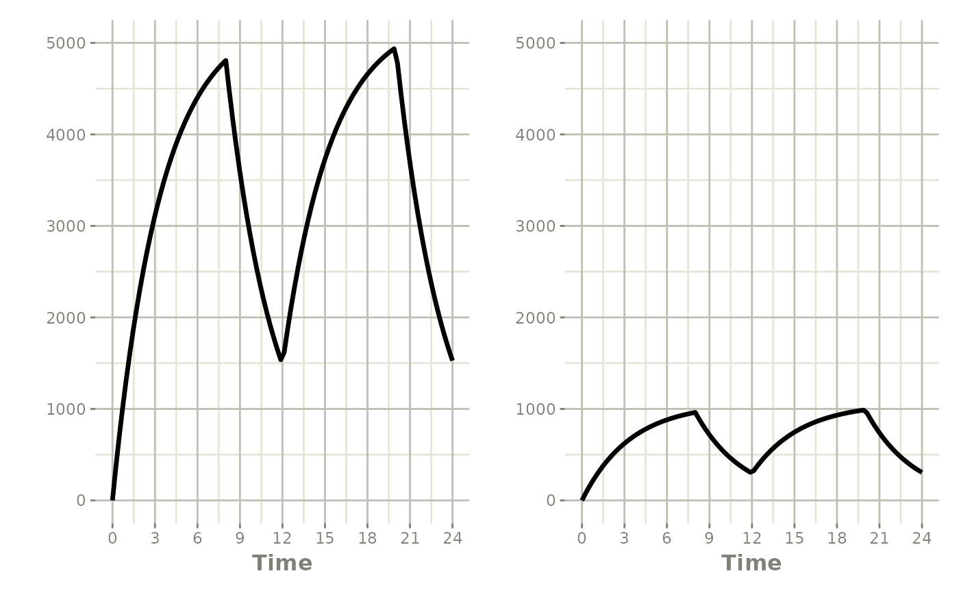

Modeled Rate and Duration of Infusion

You can model the duration, which is equivalent to NONMEM’s rate=-2.

ev <- et(timeUnits="hr") %>%
    et(amt=10000, ii=12,until=24, rate=-2) %>%
    et(seq(0, 24, length.out=100))

ev

#> -- EventTable with 101 records --
#> 1 dosing records (see x$get.dosing(); add with add.dosing or et)
#> 100 observation times (see x$get.sampling(); add with add.sampling or et)
#> multiple doses in `addl` columns, expand with x$expand(); or etExpand(x)
#> -- First part of x: --
#> # A tibble: 101 x 6
#>     time   amt rate        ii  addl evid         
#>      [h] <dbl> <rate/dur> [h] <int> <evid>       
#>  1 0        NA NA          NA    NA 0:Observation
#>  2 0     10000 -2:dur      12     2 1:Dose (Add) 
#>  3 0.242    NA NA          NA    NA 0:Observation
#>  4 0.485    NA NA          NA    NA 0:Observation
#>  5 0.727    NA NA          NA    NA 0:Observation
#>  6 0.970    NA NA          NA    NA 0:Observation
#>  7 1.21     NA NA          NA    NA 0:Observation
#>  8 1.45     NA NA          NA    NA 0:Observation
#>  9 1.70     NA NA          NA    NA 0:Observation
#> 10 1.94     NA NA          NA    NA 0:Observation
#> # i 91 more rows

rxSolve(m1, ev, c(durDepot=7)) %>% plot(depot, C2) +
    xlab("Time")

#> i parameter labels from comments are typically ignored in non-interactive mode

#> i Need to run with the source intact to parse comments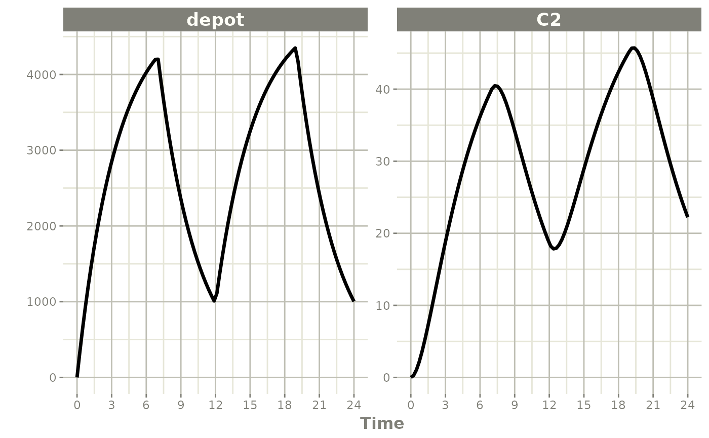

Similarly, you may also model rate. This is equivalent to NONMEM’s rate=-1 and is how rxode2’s event table specifies the data item as well.

ev <- et(timeUnits="hr") %>%
    et(amt=10000, ii=12,until=24, rate=-1) %>%
    et(seq(0, 24, length.out=100))

ev

#> -- EventTable with 101 records --
#> 1 dosing records (see x$get.dosing(); add with add.dosing or et)
#> 100 observation times (see x$get.sampling(); add with add.sampling or et)
#> multiple doses in `addl` columns, expand with x$expand(); or etExpand(x)
#> -- First part of x: --
#> # A tibble: 101 x 6
#>     time   amt rate        ii  addl evid         
#>      [h] <dbl> <rate/dur> [h] <int> <evid>       
#>  1 0        NA NA          NA    NA 0:Observation
#>  2 0     10000 -1:rate     12     2 1:Dose (Add) 
#>  3 0.242    NA NA          NA    NA 0:Observation
#>  4 0.485    NA NA          NA    NA 0:Observation
#>  5 0.727    NA NA          NA    NA 0:Observation
#>  6 0.970    NA NA          NA    NA 0:Observation
#>  7 1.21     NA NA          NA    NA 0:Observation
#>  8 1.45     NA NA          NA    NA 0:Observation
#>  9 1.70     NA NA          NA    NA 0:Observation
#> 10 1.94     NA NA          NA    NA 0:Observation
#> # i 91 more rows

rxSolve(m1, ev, c(rateDepot=10000/3)) %>% plot(depot, C2) +
    xlab("Time")

#> i parameter labels from comments are typically ignored in non-interactive mode

#> i Need to run with the source intact to parse comments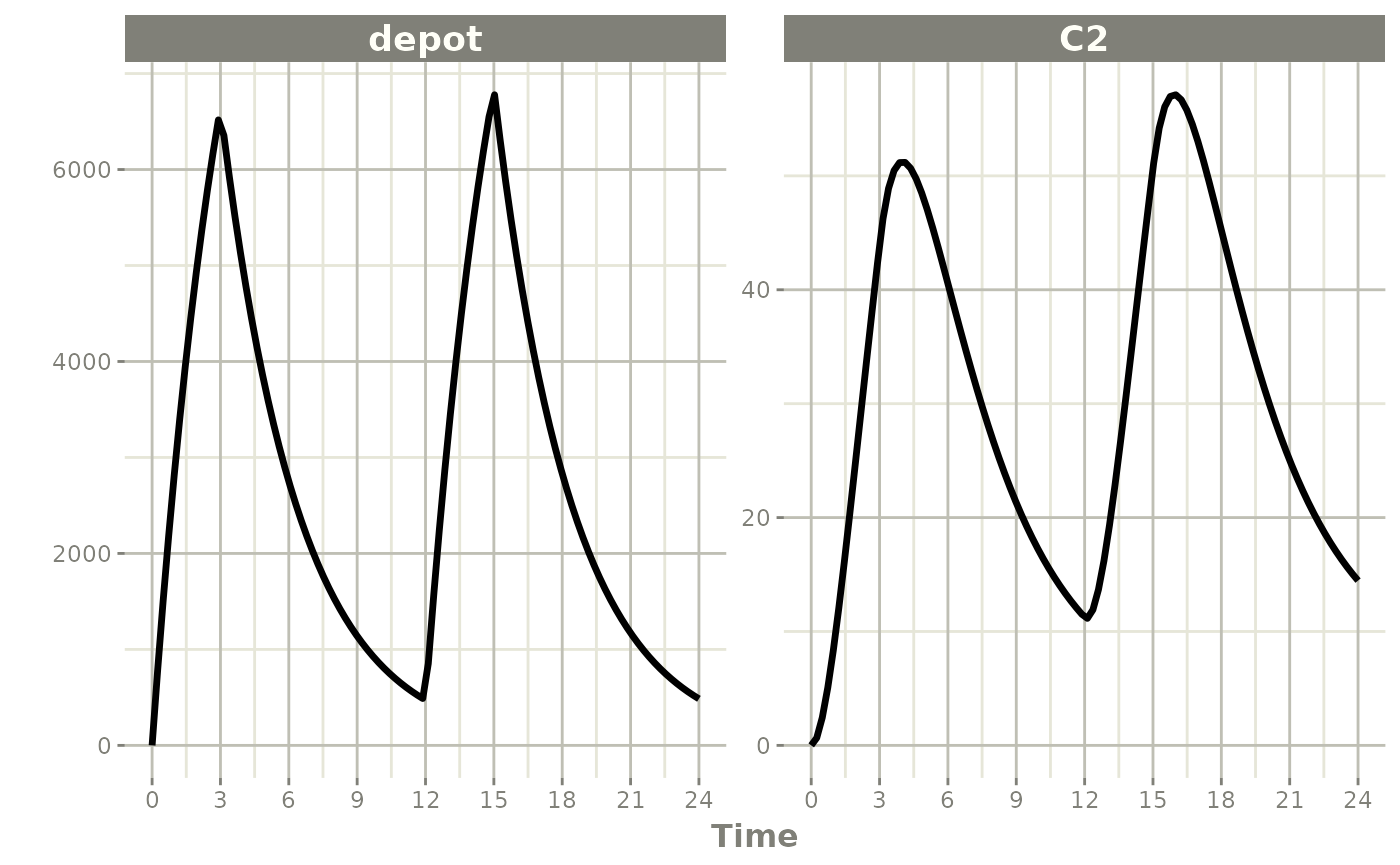

Steady State

These doses are solved until a steady state is reached with a constant inter-dose interval.

ev <- et(timeUnits="hr") %>%
    et(amt=10000, ii=12, ss=1) %>%
    et(seq(0, 24, length.out=100))

ev

#> -- EventTable with 101 records --
#> 1 dosing records (see x$get.dosing(); add with add.dosing or et)
#> 100 observation times (see x$get.sampling(); add with add.sampling or et)
#> -- First part of x: --
#> # A tibble: 101 x 5
#>     time   amt  ii evid             ss
#>      [h] <dbl> [h] <evid>        <int>
#>  1 0        NA  NA 0:Observation    NA
#>  2 0     10000  12 1:Dose (Add)      1
#>  3 0.242    NA  NA 0:Observation    NA
#>  4 0.485    NA  NA 0:Observation    NA
#>  5 0.727    NA  NA 0:Observation    NA
#>  6 0.970    NA  NA 0:Observation    NA
#>  7 1.21     NA  NA 0:Observation    NA
#>  8 1.45     NA  NA 0:Observation    NA
#>  9 1.70     NA  NA 0:Observation    NA
#> 10 1.94     NA  NA 0:Observation    NA
#> # i 91 more rows

rxSolve(m1, ev) %>% plot(C2)

#> i parameter labels from comments are typically ignored in non-interactive mode

#> i Need to run with the source intact to parse comments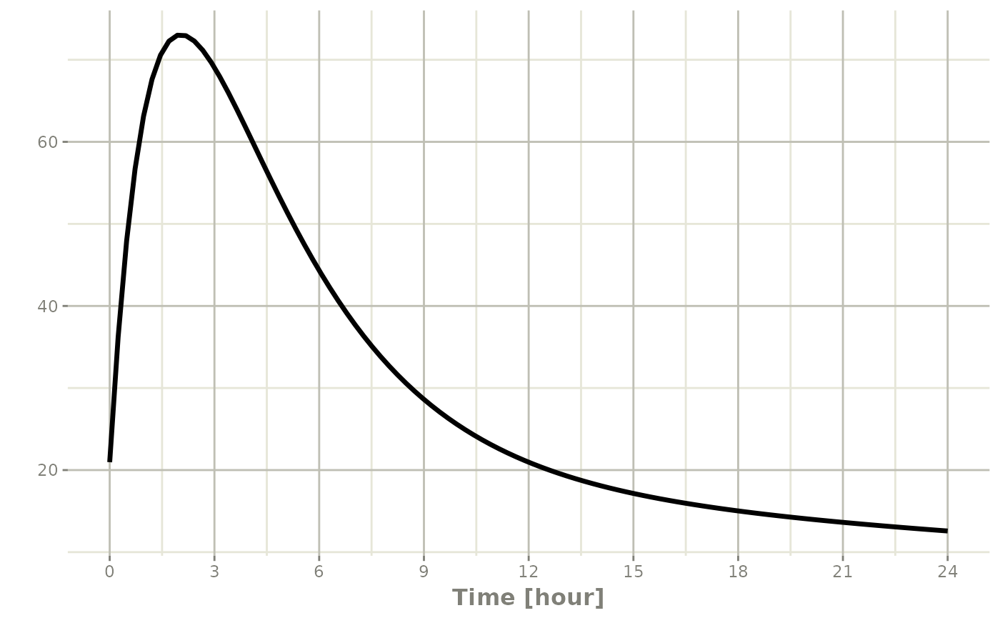

Steady state for complex dosing

By using the ss=2 flag, you can use the super-positioning principle in linear kinetics to get steady state nonstandard dosing (i.e. morning 100 mg vs evening 150 mg). This is done by:

Saving all the state values
Resetting all the states and solving the system to steady state
Adding back all the prior state values

ev <- et(timeUnits="hr") %>%
    et(amt=10000, ii=24, ss=1) %>%
    et(time=12, amt=15000, ii=24, ss=2) %>%
    et(time=24, amt=10000, ii=24, addl=3) %>%
    et(time=36, amt=15000, ii=24, addl=3) %>%
    et(seq(0, 64, length.out=500))

library(ggplot2)

rxSolve(m1, ev,maxsteps=10000) %>% plot(C2) +
  annotate("rect", xmin=0, xmax=24, ymin=-Inf, ymax=Inf,
           alpha=0.2) +
  annotate("text", x=12.5, y=7,
           label="Initial Steady State Period") +
  annotate("text", x=44,   y=7,
           label="Steady State AM/PM dosing")

#> i parameter labels from comments are typically ignored in non-interactive mode

#> i Need to run with the source intact to parse comments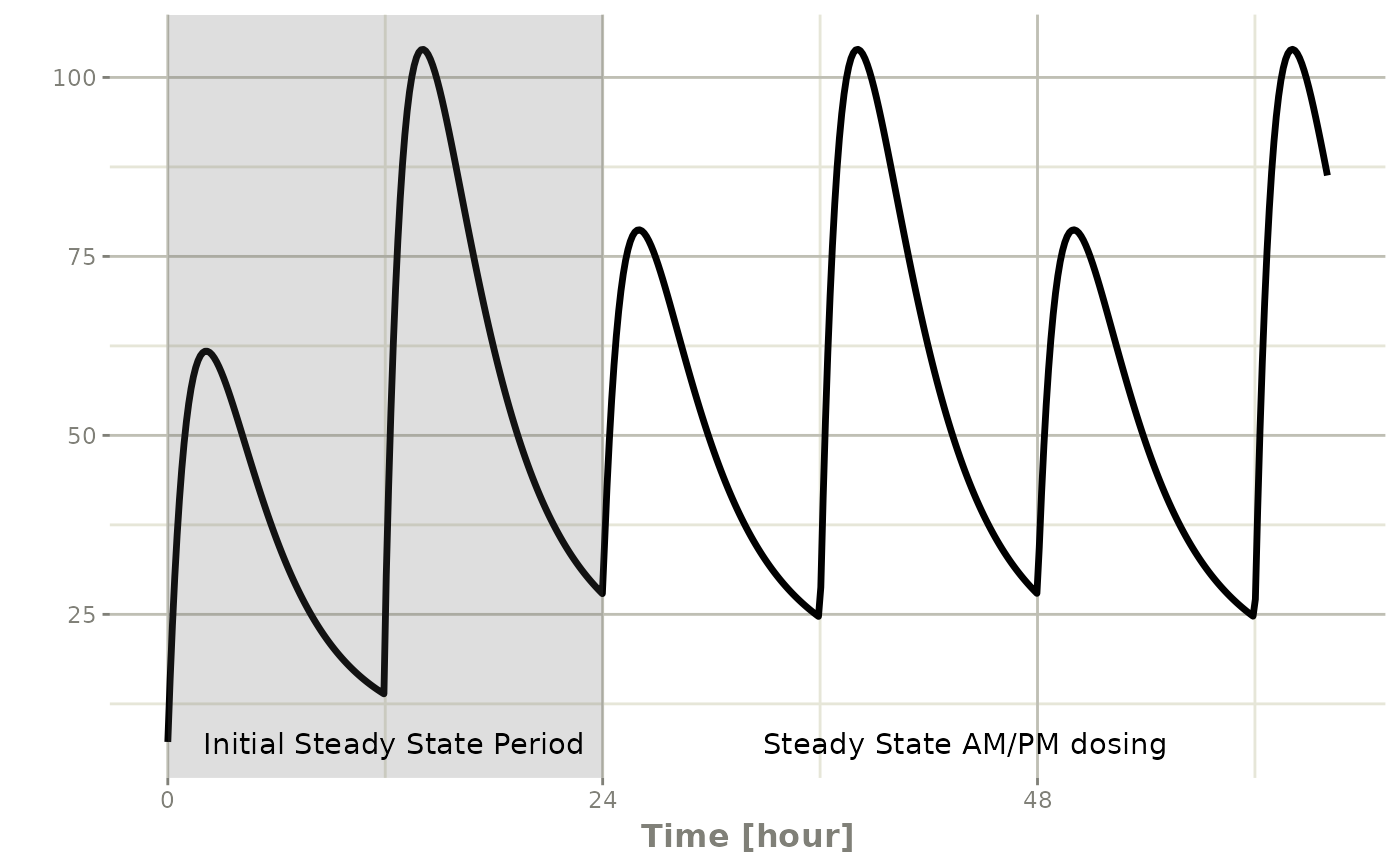

You can see that it takes a full dose cycle to reach the true complex steady state dosing.

Steady state for constant infusion or zero order processes

The last type of steady state that rxode2 supports is steady-state constant infusion rate. This can be specified the same way as NONMEM, that is:

No inter-dose interval ii=0
A steady state dose, ie ss=1
Either a positive rate (rate>0) or a estimated rate rate=-1.
A zero dose, ie amt=0
Once the steady-state constant infusion is achieved, the infusion is turned off when using this record, just like NONMEM.

Note that rate=-2 where we model the duration of infusion doesn’t make much sense since we are solving the infusion until steady state. The duration is specified by the steady state solution.

Also note that bioavailability changes on this steady state infusion also do not make sense because they neither change the rate or the duration of the steady state infusion. Hence modeled bioavailability on this type of dosing event is ignored.

Here is an example:

ev <- et(timeUnits="hr") %>%
    et(amt=0, ss=1,rate=10000/8)

p1 <- rxSolve(m1, ev) %>% plot(C2, eff)

#> i parameter labels from comments are typically ignored in non-interactive mode

#> i Need to run with the source intact to parse comments

ev <- et(timeUnits="hr") %>%
    et(amt=200000, rate=10000/8) %>%
    et(0, 250, length.out=1000)

p2 <- rxSolve(m1, ev) %>% plot(C2, eff)

#> i parameter labels from comments are typically ignored in non-interactive mode
#> i Need to run with the source intact to parse comments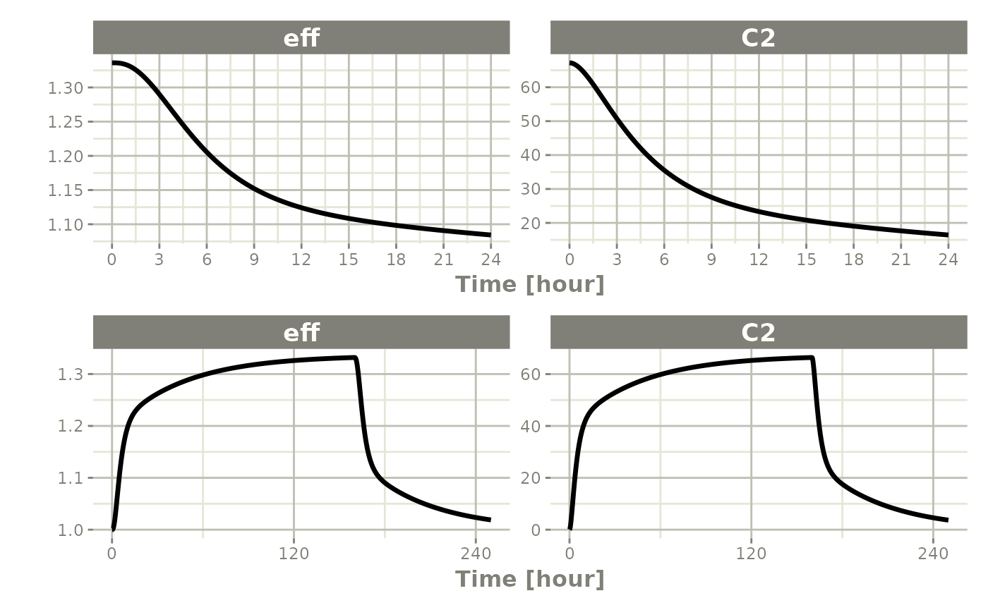

library(patchwork)

p1 / p2

Not only can this be used for PK, it can be used for steady-state disease processes.

Reset Events

Reset events are implemented by evid=3 or evid=reset, for reset and evid=4 for reset and dose.

ev <- et(timeUnits="hr") %>%
    et(amt=10000, ii=12, addl=3) %>%
    et(time=6, evid=reset) %>%
    et(seq(0, 24, length.out=100))

ev

#> -- EventTable with 102 records --
#> 2 dosing records (see x$get.dosing(); add with add.dosing or et)
#> 100 observation times (see x$get.sampling(); add with add.sampling or et)
#> multiple doses in `addl` columns, expand with x$expand(); or etExpand(x)
#> -- First part of x: --
#> # A tibble: 102 x 5
#>     time   amt  ii  addl evid         
#>      [h] <dbl> [h] <int> <evid>       
#>  1 0        NA  NA    NA 0:Observation
#>  2 0     10000  12     3 1:Dose (Add) 
#>  3 0.242    NA  NA    NA 0:Observation
#>  4 0.485    NA  NA    NA 0:Observation
#>  5 0.727    NA  NA    NA 0:Observation
#>  6 0.970    NA  NA    NA 0:Observation
#>  7 1.21     NA  NA    NA 0:Observation
#>  8 1.45     NA  NA    NA 0:Observation
#>  9 1.70     NA  NA    NA 0:Observation
#> 10 1.94     NA  NA    NA 0:Observation
#> # i 92 more rows

The solving show what happens in this system when the system is reset at 6 hours post-dose.

rxSolve(m1, ev) %>% plot(depot,C2, eff)

#> i parameter labels from comments are typically ignored in non-interactive mode

#> i Need to run with the source intact to parse comments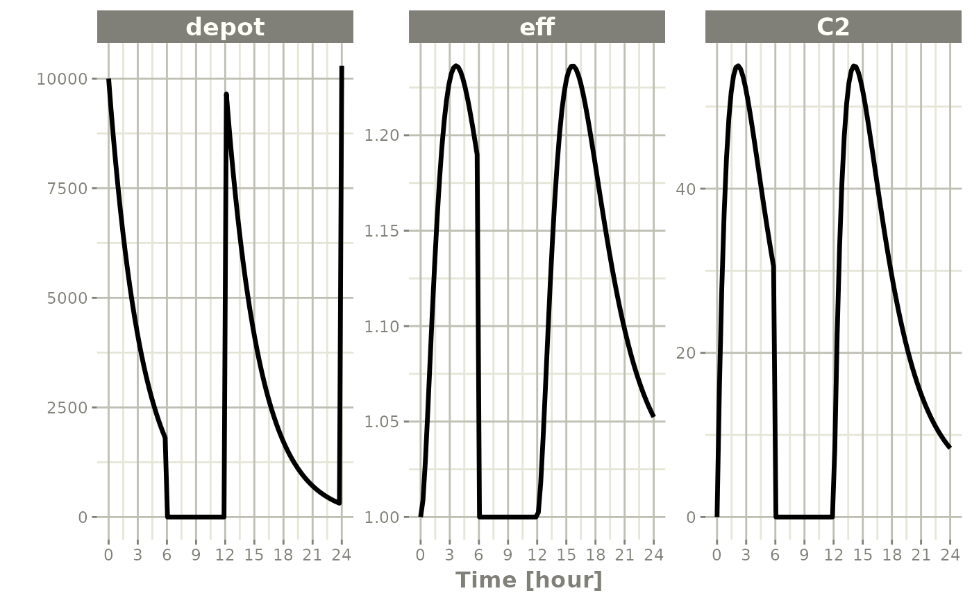

You can see all the compartments are reset to their initial values. The next dose start the dosing cycle over.

ev <- et(timeUnits="hr") %>%
    et(amt=10000, ii=12, addl=3) %>%
    et(time=6, amt=10000, evid=4) %>%
    et(seq(0, 24, length.out=100))

ev

#> -- EventTable with 102 records --
#> 2 dosing records (see x$get.dosing(); add with add.dosing or et)
#> 100 observation times (see x$get.sampling(); add with add.sampling or et)
#> multiple doses in `addl` columns, expand with x$expand(); or etExpand(x)
#> -- First part of x: --
#> # A tibble: 102 x 5
#>     time   amt  ii  addl evid         
#>      [h] <dbl> [h] <int> <evid>       
#>  1 0        NA  NA    NA 0:Observation
#>  2 0     10000  12     3 1:Dose (Add) 
#>  3 0.242    NA  NA    NA 0:Observation
#>  4 0.485    NA  NA    NA 0:Observation
#>  5 0.727    NA  NA    NA 0:Observation
#>  6 0.970    NA  NA    NA 0:Observation
#>  7 1.21     NA  NA    NA 0:Observation
#>  8 1.45     NA  NA    NA 0:Observation
#>  9 1.70     NA  NA    NA 0:Observation
#> 10 1.94     NA  NA    NA 0:Observation
#> # i 92 more rows

In this case, the whole system is reset and the dose is given

rxSolve(m1, ev) %>% plot(depot,C2, eff)

#> i parameter labels from comments are typically ignored in non-interactive mode

#> i Need to run with the source intact to parse comments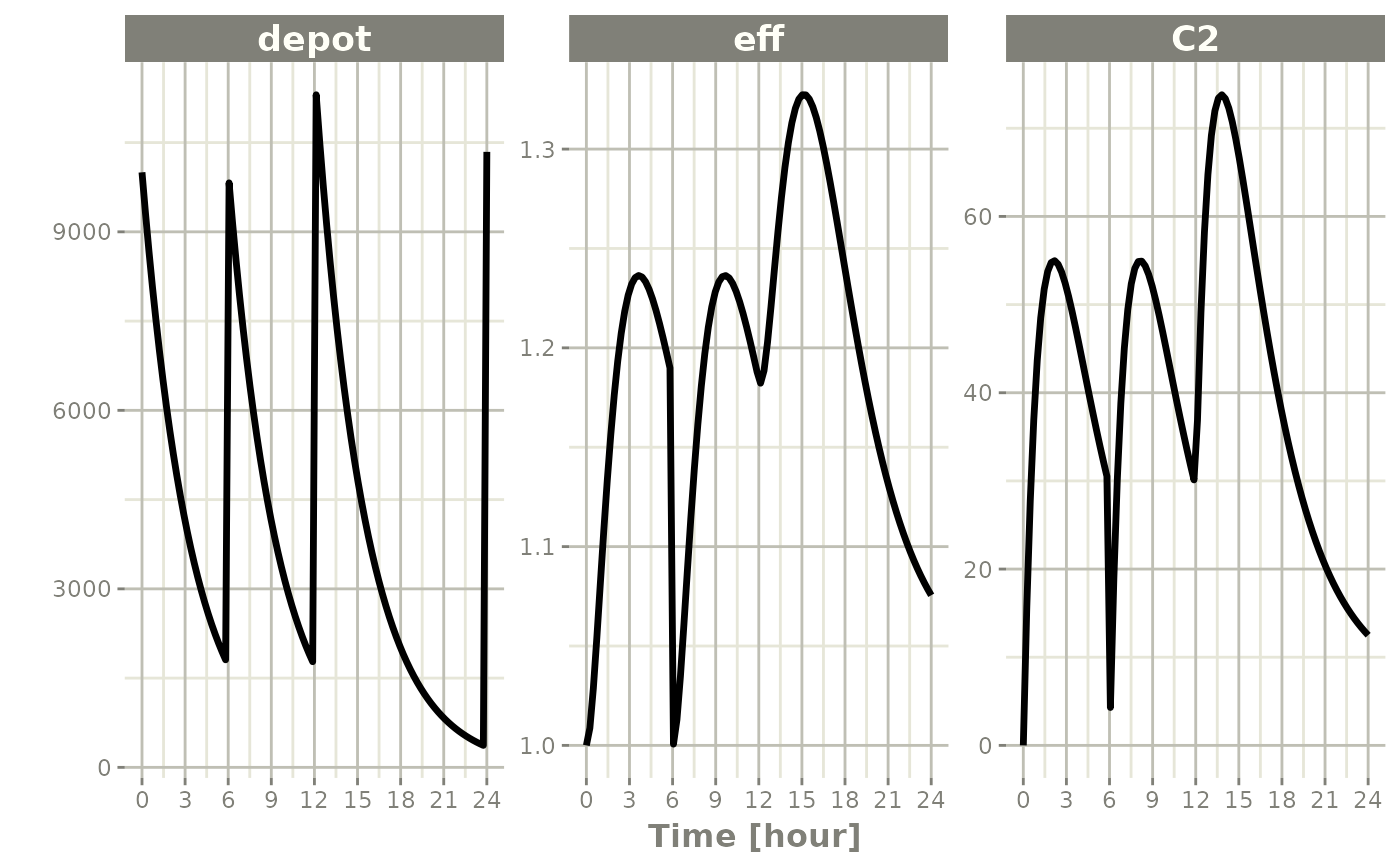

Turning off compartments

You may also turn off a compartment, which is similar to a reset event.

ev <- et(timeUnits="hr") %>%
    et(amt=10000, ii=12, addl=3) %>%
    et(time=6, cmt="-depot", evid=2) %>%
    et(seq(0, 24, length.out=100))

ev

#> -- EventTable with 102 records --
#> 2 dosing records (see x$get.dosing(); add with add.dosing or et)
#> 100 observation times (see x$get.sampling(); add with add.sampling or et)
#> multiple doses in `addl` columns, expand with x$expand(); or etExpand(x)
#> -- First part of x: --
#> # A tibble: 102 x 6
#>     time cmt         amt  ii  addl evid         
#>      [h] <chr>     <dbl> [h] <int> <evid>       
#>  1 0     (obs)        NA  NA    NA 0:Observation
#>  2 0     (default) 10000  12     3 1:Dose (Add) 
#>  3 0.242 (obs)        NA  NA    NA 0:Observation
#>  4 0.485 (obs)        NA  NA    NA 0:Observation
#>  5 0.727 (obs)        NA  NA    NA 0:Observation
#>  6 0.970 (obs)        NA  NA    NA 0:Observation
#>  7 1.21  (obs)        NA  NA    NA 0:Observation
#>  8 1.45  (obs)        NA  NA    NA 0:Observation
#>  9 1.70  (obs)        NA  NA    NA 0:Observation
#> 10 1.94  (obs)        NA  NA    NA 0:Observation
#> # i 92 more rows

Solving shows what this does in the system:

rxSolve(m1, ev) %>% plot(depot,C2, eff)

#> i parameter labels from comments are typically ignored in non-interactive mode

#> i Need to run with the source intact to parse comments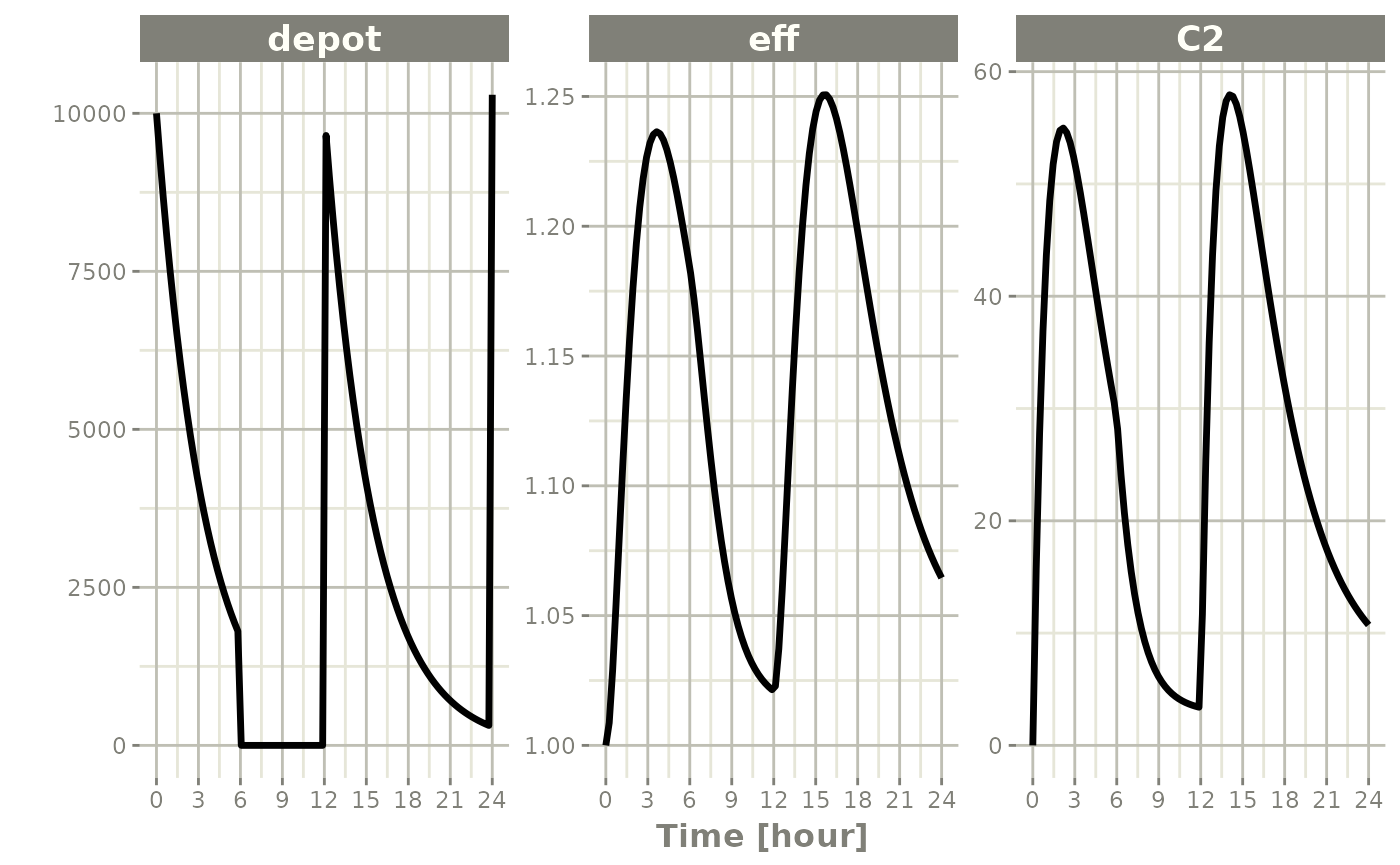

In this case, the depot is turned off, and the depot compartment concentrations are set to the initial values but the other compartment concentrations/levels are not reset. When another dose to the depot is administered the depot compartment is turned back on.

Note that a dose to a compartment only turns back on the compartment that was dosed. Hence if you turn off the effect compartment, it continues to be off after another dose to the depot.

ev <- et(timeUnits="hr") %>%
    et(amt=10000, ii=12, addl=3) %>%
    et(time=6, cmt="-eff", evid=2) %>%
    et(seq(0, 24, length.out=100))

rxSolve(m1, ev) %>% plot(depot,C2, eff)

#> i parameter labels from comments are typically ignored in non-interactive mode

#> i Need to run with the source intact to parse comments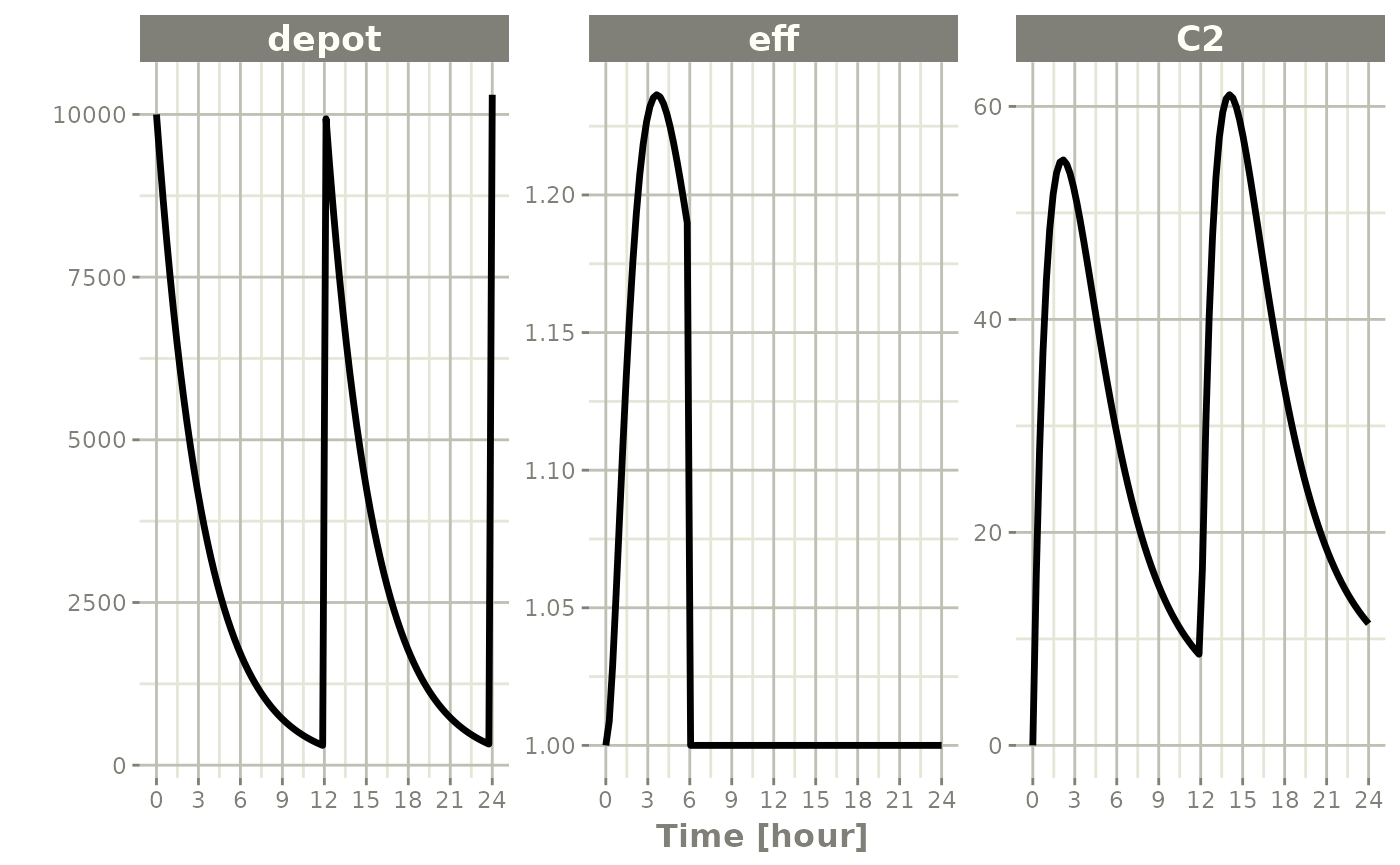

To turn back on the compartment, a zero-dose to the compartment or a evid=2 with the compartment would be needed.

ev <- et(timeUnits="hr") %>%
    et(amt=10000, ii=12, addl=3) %>%
    et(time=6, cmt="-eff", evid=2) %>%
    et(time=12,cmt="eff",evid=2) %>%
    et(seq(0, 24, length.out=100))

rxSolve(m1, ev) %>% plot(depot,C2, eff)

#> i parameter labels from comments are typically ignored in non-interactive mode

#> i Need to run with the source intact to parse comments

2025-05-16