Numerical Derivatives of (x,y) Data (via Smoothing Splines)

Compute the numerical first or 2nd derivatives of $f()$ given observations (x[i], y ~= f(x[i])).

D1tr is the trivial discrete first derivative using simple difference ratios, whereas D1ss and D2ss use cubic smoothing splines (see smooth.spline) to estimate first or second derivatives, respectively.

D2ss first uses smooth.spline for the first derivative $f'()$ and then applies the same to the predicted values $\hat f'(t_i)$ (where $t_i$ are the values of xout) to find $\hat f''(t_i)$.

Usage

D1tr(y, x = 1)

D1ss(x, y, xout = x, spar.offset = 0.1384, spl.spar=NULL)
D2ss(x, y, xout = x, spar.offset = 0.1384, spl.spar=NULL)

Arguments

x,y: numeric vectors of same length, supposedly from a model y ~ f(x). For D1tr(), x can have length one and then gets the meaning of $h = \Delta x$.
xout: abscissa values at which to evaluate the derivatives.
spar.offset: numeric fudge added to the smoothing parameter(s), see spl.par below. Note that the current default is there for historical reasons only, and we often would recommend to use spar.offset = 0 instead.
spl.spar: direct smoothing parameter(s) for smooth.spline. If it is NULL (as per default), the smoothing parameter used will be spar.offset + sp$spar, where sp$spar is the GCV estimated smoothing parameter for both smooths, see smooth.spline.

Details

It is well known that for derivative estimation, the optimal smoothing parameter is larger (more smoothing needed) than for the function itself. spar.offset is really just a fudge offset added to the smoothing parameters. Note that in R's implementation of smooth.spline, spar is really on the $\log\lambda$ scale.

Value

D1tr() and D1ss() return a numeric vector of the length of y or xout, respectively.

D2ss() returns a list with components

x: the abscissae values (= xout) at which the derivative(s) are evaluated.
y: estimated values of $f''(x_i)$.
spl.spar: numeric vector of length 2, contain the spar arguments to the two smooth.spline calls.
spar.offset: as specified on input (maybe rep()eated to length 2).

Author

Martin Maechler, in 1992 (for S).

Examples


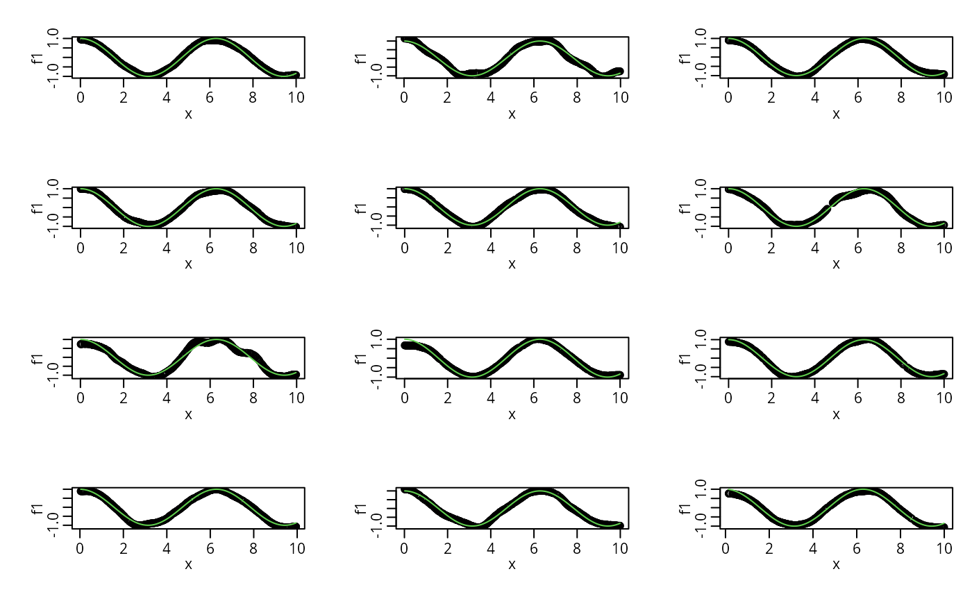
## First Derivative  --- spar.off = 0  ok "asymptotically" (?)
set.seed(330)
mult.fig(12)
for(i in 1:12) {
  x <- runif(500, 0,10); y <- sin(x) + rnorm(500)/4
  f1 <- D1ss(x=x,y=y, spar.off=0.0)
  plot(x,f1, ylim = range(c(-1,1,f1)))
  curve(cos(x), col=3, add= TRUE)
}


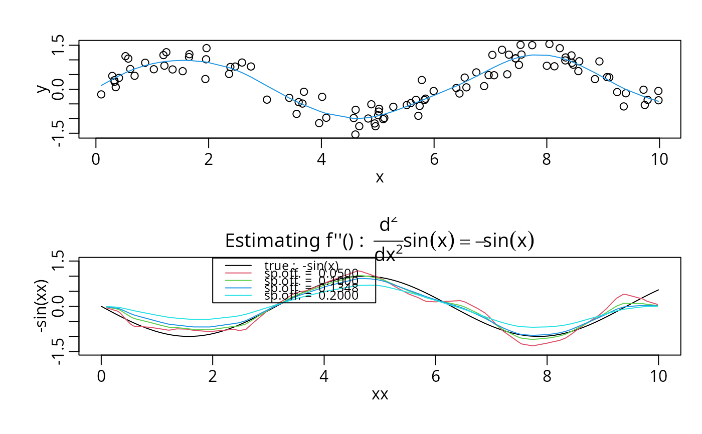
 set.seed(8840)
 x <- runif(100, 0,10)
 y <- sin(x) + rnorm(100)/4

 op <- par(mfrow = c(2,1))
 plot(x,y)
 lines(ss <- smooth.spline(x,y), col = 4)
 str(ss[c("df", "spar")])
#> List of 2
#>  $ df  : num 10.3
#>  $ spar: num 0.716
 xx <- seq(0,10, len=201)
 plot(xx, -sin(xx), type = 'l', ylim = c(-1.5,1.5))
 title(expression("Estimating f''() :  " * frac(d^2,dx^2) * sin(x) == -sin(x)))
 offs <- c(0.05, 0.1, 0.1348, 0.2)
 i <- 1
 for(off in offs) {
   d12 <- D2ss(x,y, spar.offset = off)
   lines(d12, col = i <- i+1)
 }
 legend(2,1.6, c("true :  -sin(x)",paste("sp.off. = ", format(offs))), lwd=1,
        col = 1:(1+length(offs)), cex = 0.8, bg = NA)

 par(op)