Tukey-Anscombe Plot (Residual vs. Fitted) of a Linear Model
TA.plot.RdFrom a linear (or glm) model fitted, produce the so-called Tukey-Anscombe plot. Useful (optional) additions include: 0-line, lowess smooth, 2sigma lines, and automatic labeling of observations.
Usage
TA.plot(lm.res,
        fit= fitted(lm.res), res= residuals(lm.res, type="pearson"),
        labels= NULL, main= mk.main(), xlab = "Fitted values",
        draw.smooth= n >= 10, show.call = TRUE, show.2sigma= TRUE,
        lo.iter = NULL, lo.cex= NULL,
        par0line  = list(lty = 2, col = "gray"),
        parSmooth = list(lwd = 1.5, lty = 4, col = 2),
        parSigma  = list(lwd = 1.2, lty = 3, col = 4),
        verbose = FALSE,
        ...)
Arguments
- lm.res
- fit
fitted values; you probably want the default here.
- res
residuals to use. Default: Weighted ("Pearson") residuals if weights have been used for the model fit.
- labels
strings to use as plotting symbols for each point. Default(
NULL): extract observations' names or use its sequence number. Use, e.g., "*" to get simple*symbols.- main
main title to plot. Default: sophisticated, resulting in something like "Tukey-Anscombe Plot of : y ~ x" constructed from
lm.res $ call.- xlab
x-axis label for plot.
- draw.smooth
logical; if
TRUE, draw alowesssmoother (with automatic smoothing fraction).- show.call
logical; if
TRUE, write the "call"ing syntax with which the fit was done.- show.2sigma
logical; if
TRUE, draw horizontal lines at \(\pm 2\sigma\) where \(\sigma\) ismad(resid).- lo.iter
positive integer, giving the number of lowess robustness iterations. The default depends on the model and is
0for non Gaussianglm's.- lo.cex
character expansion ("cex") for lowess and other marginal texts.
- par0line
a list of arguments (with reasonable defaults) to be passed to
abline(.)when drawing the x-axis, i.e., the \(y = 0\) line.- parSmooth, parSigma
each a list of arguments (with reasonable default) for drawing the smooth curve (if
draw.smoothis true), or the horizontal sigma boundaries (ifshow.2sigmais true) respectively.- verbose
logical indicating if some construction details should be reported (
print()ed).- ...
further graphical parameters are passed to
n.plot(.).
Author
Martin Maechler, Seminar fuer Statistik, ETH Zurich, Switzerland; maechler@stat.math.ethz.ch
See also
plot.lm which also does a QQ normal plot and more.
Examples
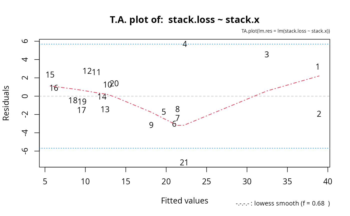
data(stackloss)
TA.plot(lm(stack.loss ~ stack.x))
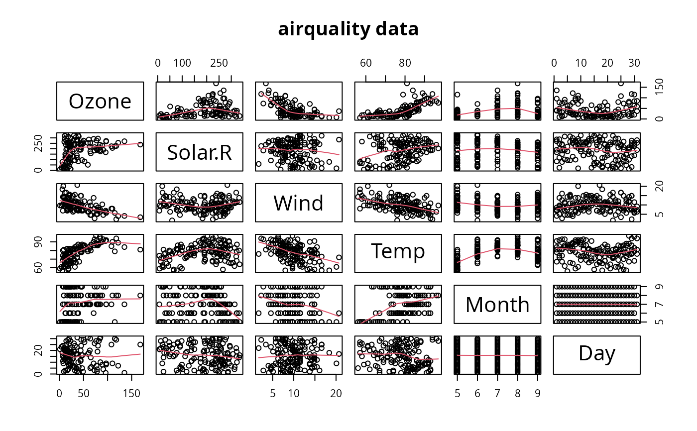
 example(airquality)
#>
#> arqlty> require(graphics)
#>
#> arqlty> pairs(airquality, panel = panel.smooth, main = "airquality data")
example(airquality)
#>
#> arqlty> require(graphics)
#>
#> arqlty> pairs(airquality, panel = panel.smooth, main = "airquality data")
 summary(lmO <- lm(Ozone ~ ., data= airquality))
#>
#> Call:
#> lm(formula = Ozone ~ ., data = airquality)
#>
#> Residuals:
#> Min 1Q Median 3Q Max
#> -37.014 -12.284 -3.302 8.454 95.348
#>
#> Coefficients:
#> Estimate Std. Error t value Pr(>|t|)
#> (Intercept) -64.11632 23.48249 -2.730 0.00742 **
#> Solar.R 0.05027 0.02342 2.147 0.03411 *
#> Wind -3.31844 0.64451 -5.149 1.23e-06 ***
#> Temp 1.89579 0.27389 6.922 3.66e-10 ***
#> Month -3.03996 1.51346 -2.009 0.04714 *
#> Day 0.27388 0.22967 1.192 0.23576
#> ---
#> Signif. codes: 0 ‘***’ 0.001 ‘**’ 0.01 ‘*’ 0.05 ‘.’ 0.1 ‘ ’ 1
#>
#> Residual standard error: 20.86 on 105 degrees of freedom
#> (42 observations deleted due to missingness)
#> Multiple R-squared: 0.6249, Adjusted R-squared: 0.6071
#> F-statistic: 34.99 on 5 and 105 DF, p-value: < 2.2e-16
#>
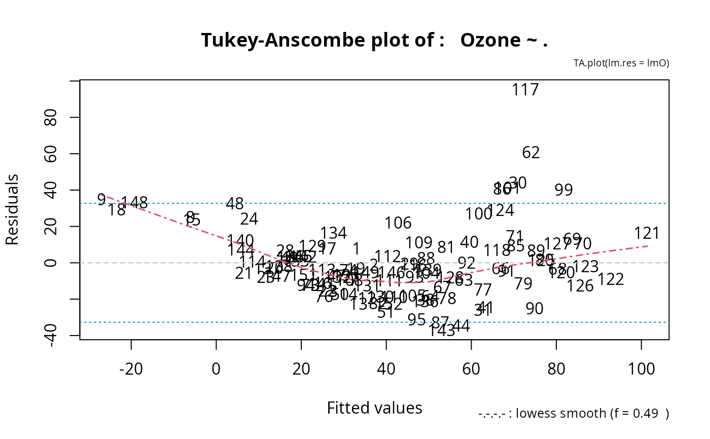
TA.plot(lmO)
summary(lmO <- lm(Ozone ~ ., data= airquality))
#>
#> Call:
#> lm(formula = Ozone ~ ., data = airquality)
#>
#> Residuals:
#> Min 1Q Median 3Q Max
#> -37.014 -12.284 -3.302 8.454 95.348
#>
#> Coefficients:
#> Estimate Std. Error t value Pr(>|t|)
#> (Intercept) -64.11632 23.48249 -2.730 0.00742 **
#> Solar.R 0.05027 0.02342 2.147 0.03411 *
#> Wind -3.31844 0.64451 -5.149 1.23e-06 ***
#> Temp 1.89579 0.27389 6.922 3.66e-10 ***
#> Month -3.03996 1.51346 -2.009 0.04714 *
#> Day 0.27388 0.22967 1.192 0.23576
#> ---
#> Signif. codes: 0 ‘***’ 0.001 ‘**’ 0.01 ‘*’ 0.05 ‘.’ 0.1 ‘ ’ 1
#>
#> Residual standard error: 20.86 on 105 degrees of freedom
#> (42 observations deleted due to missingness)
#> Multiple R-squared: 0.6249, Adjusted R-squared: 0.6071
#> F-statistic: 34.99 on 5 and 105 DF, p-value: < 2.2e-16
#>
TA.plot(lmO)
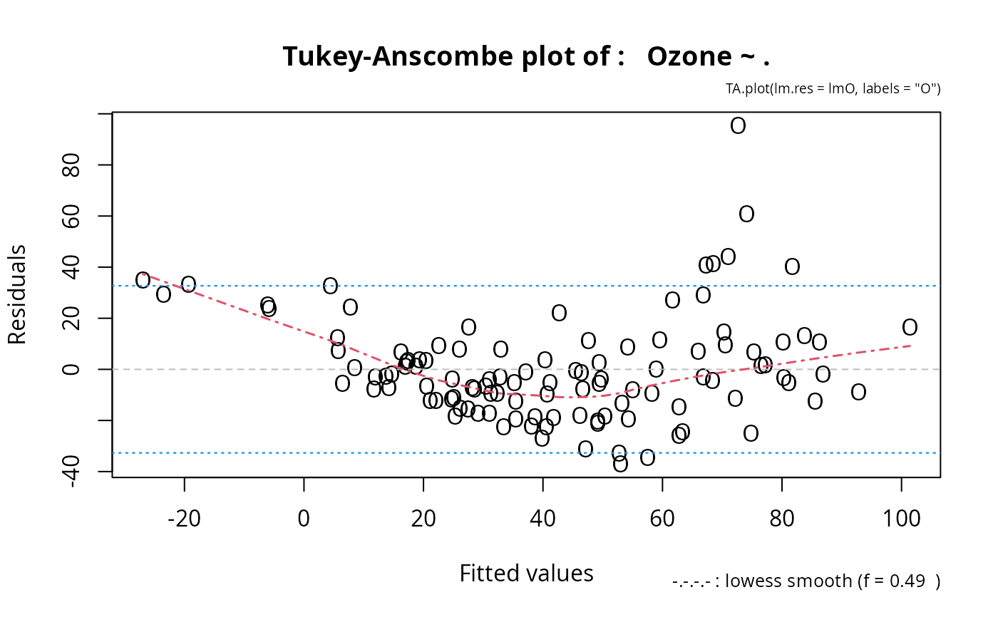
 TA.plot(lmO, label = "O") # instead of case numbers
 if(FALSE) {
TA.plot(lm(cost ~ age+type+car.age, claims, weights=number, na.action=na.omit))
}
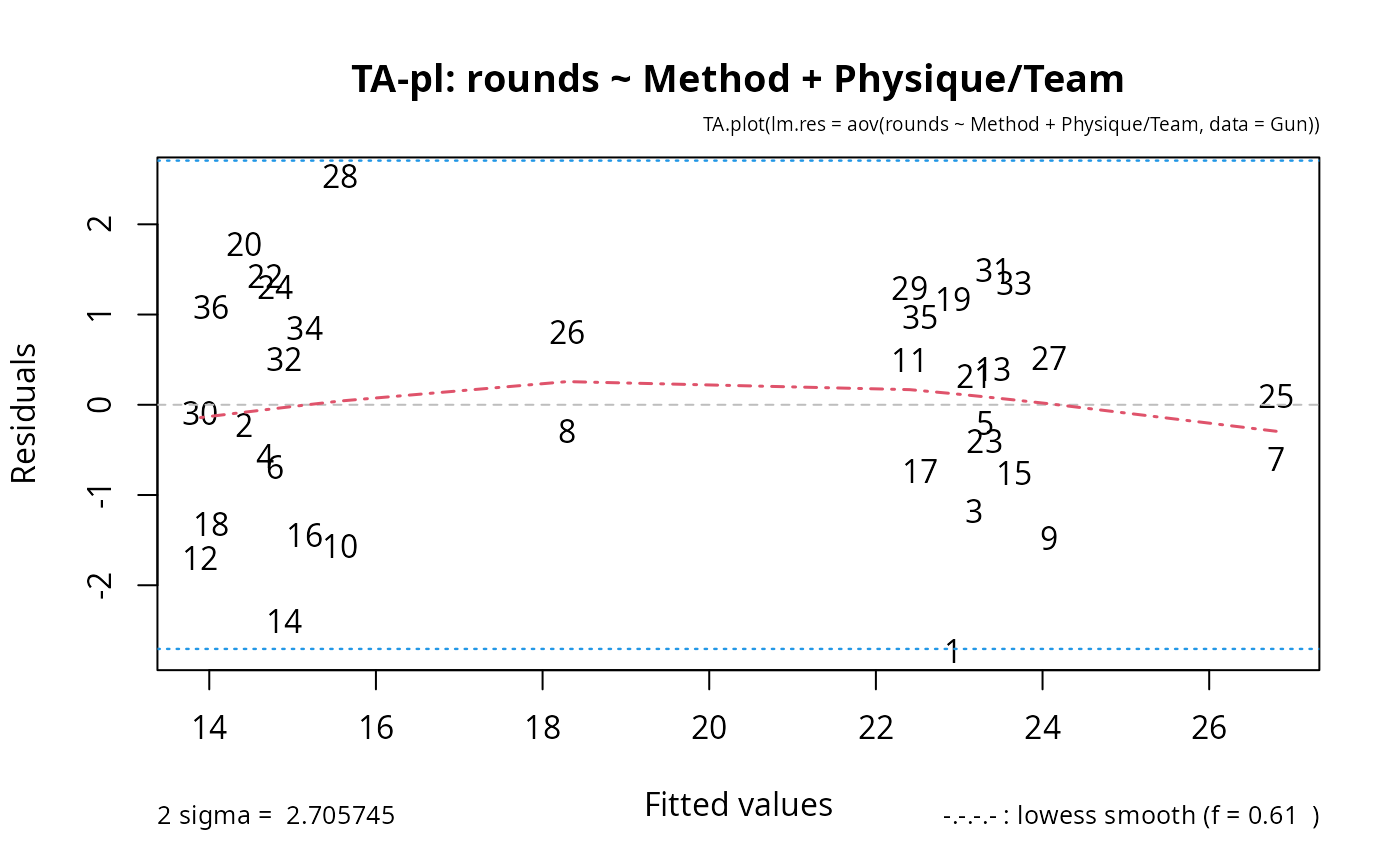
##--- for aov(.) : -------------
data(Gun, package = "nlme")
TA.plot( aov(rounds ~ Method + Physique/Team, data = Gun))
if(FALSE) {
TA.plot(lm(cost ~ age+type+car.age, claims, weights=number, na.action=na.omit))
}
##--- for aov(.) : -------------
data(Gun, package = "nlme")
TA.plot( aov(rounds ~ Method + Physique/Team, data = Gun))
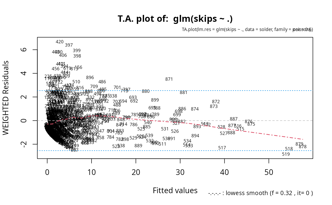
 ##--- Not so clear what it means for GLM, but: ------
if(require(rpart)) { # for the two datasets only
data(solder, package = "rpart")
TA.plot(glm(skips ~ ., data = solder, family = poisson), cex= .6)
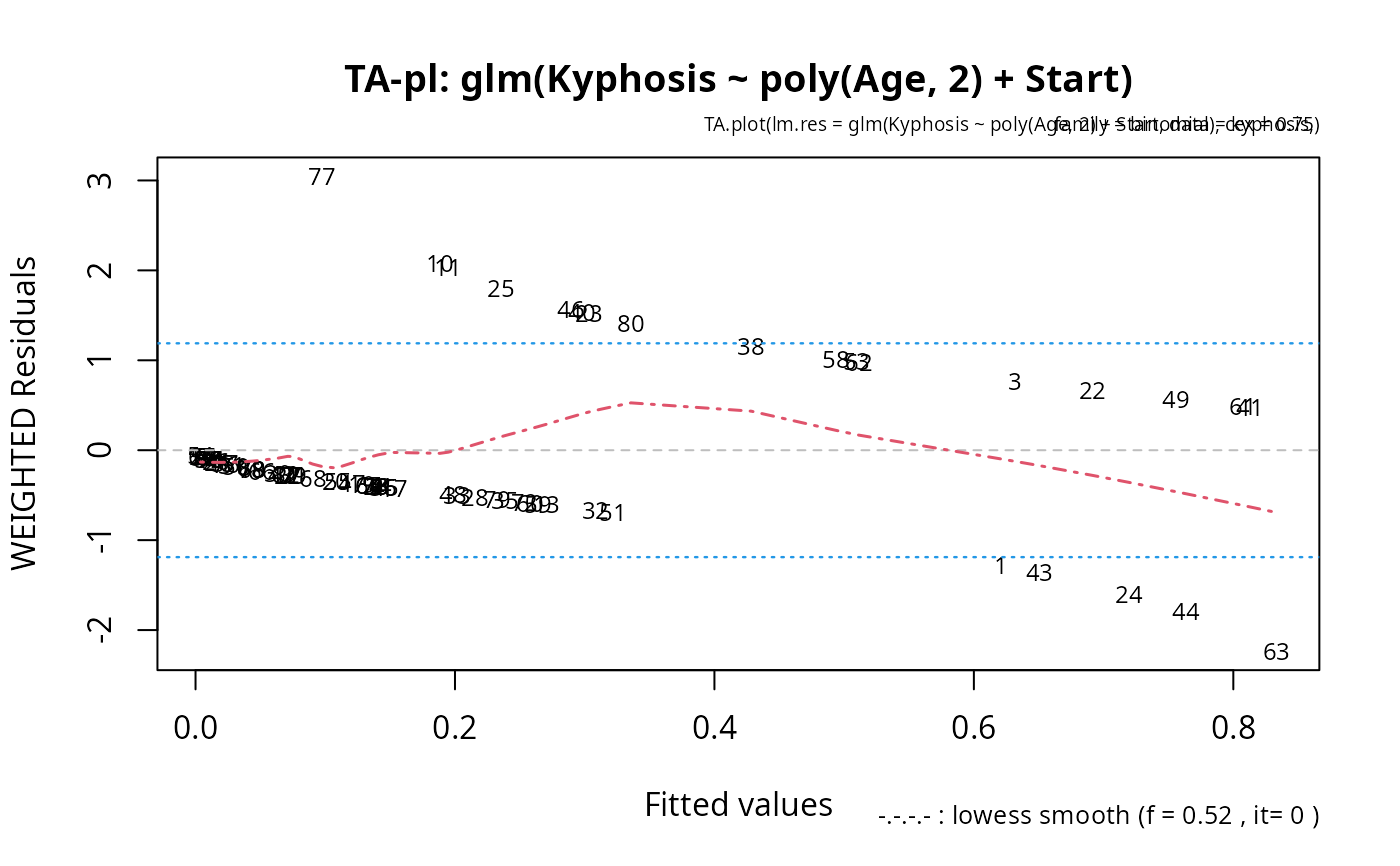
data(kyphosis, package = "rpart")
TA.plot(glm(Kyphosis ~ poly(Age,2) + Start, data=kyphosis, family = binomial),
cex=.75) # smaller title and plotting characters
}
#> Loading required package: rpart
##--- Not so clear what it means for GLM, but: ------
if(require(rpart)) { # for the two datasets only
data(solder, package = "rpart")
TA.plot(glm(skips ~ ., data = solder, family = poisson), cex= .6)
data(kyphosis, package = "rpart")
TA.plot(glm(Kyphosis ~ poly(Age,2) + Start, data=kyphosis, family = binomial),
cex=.75) # smaller title and plotting characters
}
#> Loading required package: rpart