Diagonal Discriminant Analysis

This function implements a simple Gaussian maximum likelihood discriminant rule, for diagonal class covariance matrices.

In machine learning lingo, this is called “Naive Bayes” (for continuous predictors). Note that naive Bayes is more general, as it models discrete predictors as multinomial, i.e., binary predictor variables as Binomial / Bernoulli.

Usage

dDA(x, cll, pool = TRUE)
# S3 method for class 'dDA'
predict(object, newdata, pool = object$pool, ...)
# S3 method for class 'dDA'
print(x, ...)

diagDA(ls, cll, ts, pool = TRUE)

Arguments

x,ls: learning set data matrix, with rows corresponding to cases (e.g., mRNA samples) and columns to predictor variables (e.g., genes).
cll: class labels for learning set, must be consecutive integers.
object: object of class dDA.
ts, newdata: test set (prediction) data matrix, with rows corresponding to cases and columns to predictor variables.
pool: logical flag. If true (by default), the covariance matrices are assumed to be constant across classes and the discriminant rule is linear in the data. Otherwise (pool= FALSE), the covariance matrices may vary across classes and the discriminant rule is quadratic in the data.
...: further arguments passed to and from methods.

Value

dDA() returns an object of class dDA for which there are print and predict methods. The latter returns the same as diagDA():

diagDA() returns an integer vector of class predictions for the test set.

References

S. Dudoit, J. Fridlyand, and T. P. Speed. (2000) Comparison of Discrimination Methods for the Classification of Tumors Using Gene Expression Data. (Statistics, UC Berkeley, June 2000, Tech Report #576)

Author

Sandrine Dudoit, sandrine@stat.berkeley.edu and
Jane Fridlyand, janef@stat.berkeley.edu originally wrote stat.diag.da() in CRAN package sma which was modified for speedup by Martin Maechler maechler@R-project.org who also introduced dDA etc.

Examples

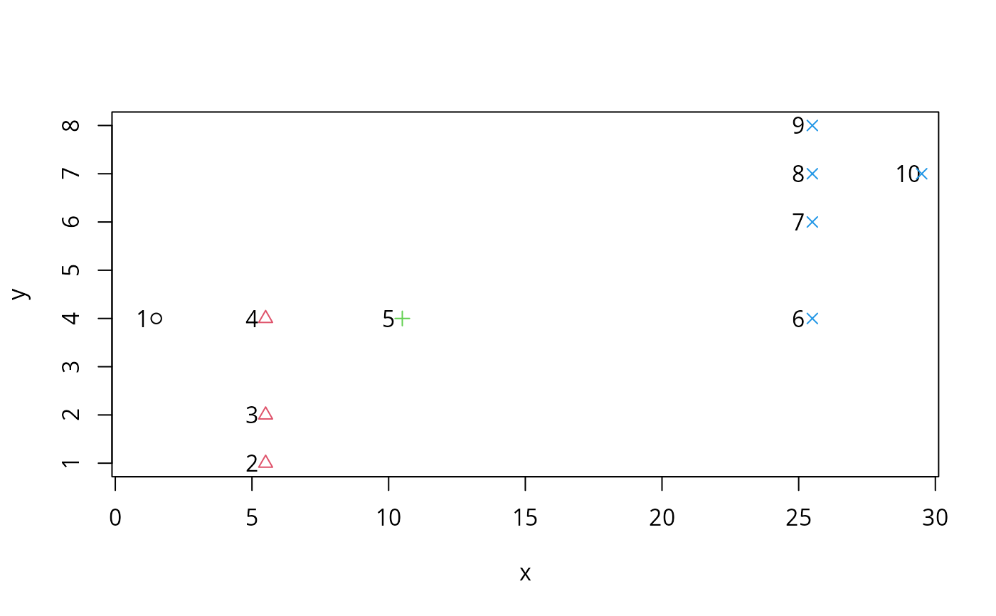
## two artificial examples by Andreas Greutert:
d1 <- data.frame(x = c(1, 5, 5, 5, 10, 25, 25, 25, 25, 29),
                 y = c(4, 1, 2, 4,  4,  4,     6:8,     7))
n.plot(d1)
library(cluster)
(cl1P <- pam(d1,k=4)$cluster) # 4 surprising clusters
#>  [1] 1 2 2 2 3 4 4 4 4 4
with(d1, points(x+0.5, y, col = cl1P, pch =cl1P))


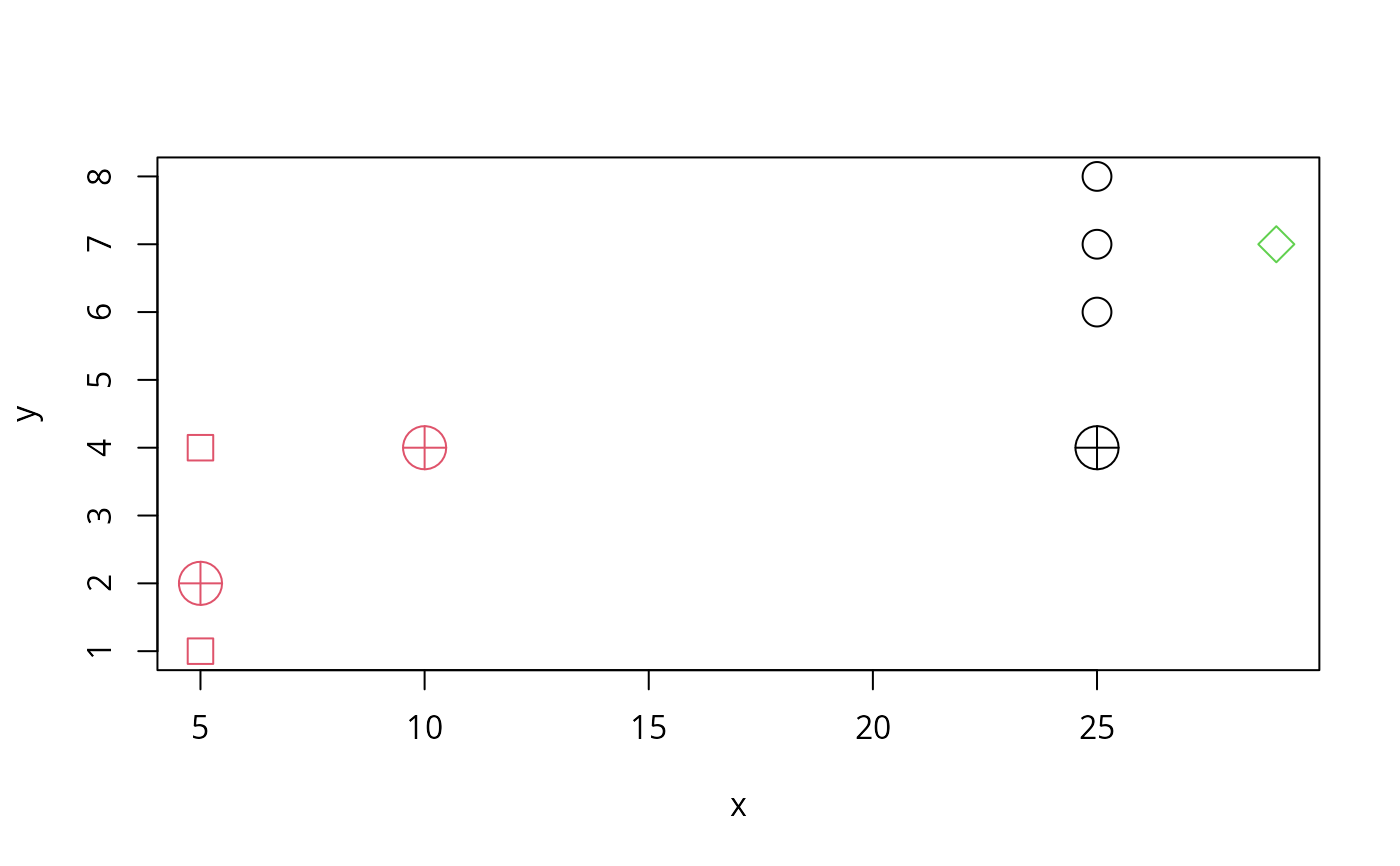
i1 <- c(1,3,5,6)
tr1 <- d1[-i1,]
cl1. <- c(1,2,1,2,1,3)
cl1  <- c(2,2,1,1,1,3)
plot(tr1, cex=2, col = cl1, pch = 20+cl1)
(dd.<- diagDA(tr1, cl1., ts = d1[ i1,]))# ok
#> [1] 2 2 2 1
(dd <- diagDA(tr1, cl1 , ts = d1[ i1,]))# ok, too!
#> [1] 2 2 2 1
points(d1[ i1,], pch = 10, cex=3, col = dd)


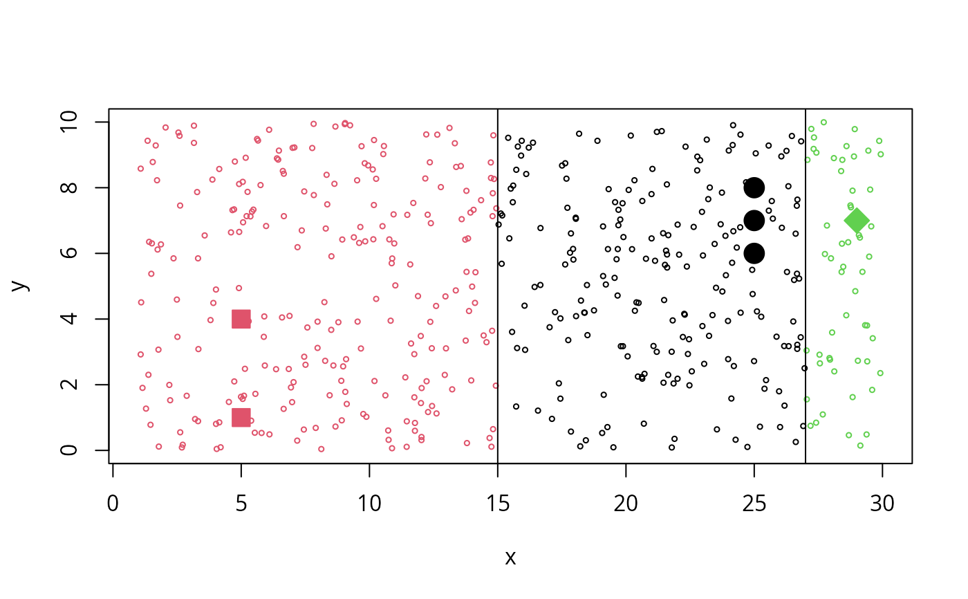
## use new fit + predict instead :
(r1 <- dDA(tr1, cl1))
#> Linear (pooled var) Diagonal Discriminant Analysis,
#>   dDA(x = tr1, cll = cl1) 
#>   (n= 6) x (p= 2) data in K=3 classes of [3, 2, 1] observations each
#> 
(r1.<- dDA(tr1, cl1.))
#> Linear (pooled var) Diagonal Discriminant Analysis,
#>   dDA(x = tr1, cll = cl1.) 
#>   (n= 6) x (p= 2) data in K=3 classes of [3, 2, 1] observations each
#> 
stopifnot(dd == predict(r1,  new = d1[ i1,]),
          dd.== predict(r1., new = d1[ i1,]))

plot(tr1, cex=2, col = cl1, bg = cl1, pch = 20+cl1,
     xlim=c(1,30), ylim= c(0,10))
xy <- cbind(x= runif(500, min=1,max=30), y = runif(500, min=0, max=10))
points(xy, cex= 0.5, col = predict(r1, new = xy))
abline(v=c( mean(c(5,25)), mean(c(25,29))))


## example where one variable xj has  Var(xj) = 0:
x4 <- matrix(c(2:4,7, 6,8,5,6,  7,2,3,1, 7,7,7,7), ncol=4)
y <- c(2,2, 1,1)
m4.1 <- dDA(x4, y, pool = FALSE)
m4.2 <- dDA(x4, y, pool = TRUE)
xx <- matrix(c(3,7,5,7), ncol=4)
predict(m4.1, xx)## gave integer(0) previously
#> [1] 2
predict(m4.2, xx)
#> [1] 2