xgx_stat_ci returns a ggplot layer plotting mean +/- confidence
intervals
Arguments
- mapping
Set of aesthetic mappings created by `aes` or `aes_`. If specified and `inherit.aes = TRUE` (the default), it is combined with the default mapping at the top level of the plot. You must supply mapping if there is no plot mapping.
- data
The data to be displayed in this layer. There are three options:
If NULL, the default, the data is inherited from the plot data as specified in the call to ggplot.
A data.frame, or other object, will override the plot data. All objects will be fortified to produce a data frame. See fortify for which variables will be created.
A function will be called with a single argument, the plot data. The return value must be a data.frame., and will be used as the layer data.
- conf_level
The percentile for the confidence interval (should fall between 0 and 1). The default is 0.95, which corresponds to a 95 percent confidence interval.
- distribution
The distribution which the data follow, used for calculating confidence intervals. The options are "normal", "lognormal", and "binomial". The "normal" option will use the Student t Distribution to calculate confidence intervals, the "lognormal" option will transform data to the log space first. The "binomial" option will use the
binom.exactfunction to calculate the confidence intervals. Note: binomial data must be numeric and contain only 1's and 0's.- bins
number of bins to cut up the x data, cuts data into quantiles.
- breaks
breaks to cut up the x data, if this option is used, bins is ignored
- geom
Use to override the default geom. Can be a list of multiple geoms, e.g. list("point","line","errorbar"), which is the default.
- position
Position adjustment, either as a string, or the result of a call to a position adjustment function.
- fun.args
Optional additional arguments passed on to the functions.
- fun.data
A function that is given the complete data and should return a data frame with variables ymin, y, and ymax.
- na.rm
If FALSE, the default, missing values are removed with a warning. If TRUE, missing values are silently removed.
- orientation
The orientation of the layer, passed on to ggplot2::stat_summary. Only implemented for ggplot2 v.3.3.0 and later. The default ("x") summarizes y values over x values (same behavior as ggplot2 v.3.2.1 or earlier). Setting
orientation = "y"will summarize x values over y values, which may be useful in some situations where you want to flip the axes, e.g. to create forest plots. Settingorientation = NAwill try to automatically determine the orientation from the aesthetic mapping (this is more stable for ggplot2 v.3.3.2 compared to v.3.3.0). Seestat_summary(v.3.3.0 or greater) for more information.- show.legend
logical. Should this layer be included in the legends? NA, the default, includes if any aesthetics are mapped. FALSE never includes, and TRUE always includes.
- inherit.aes
If FALSE, overrides the default aesthetics, rather than combining with them. This is most useful for helper functions that define both data and aesthetics and shouldn't inherit behaviour from the default plot specification, e.g. borders.
- ...
other arguments passed on to layer. These are often aesthetics, used to set an aesthetic to a fixed value, like color = "red" or size = 3. They may also be parameters to the paired geom/stat.
Details
This function can be used to generate mean +/- confidence interval plots for different distributions, and multiple geoms with a single function call.
Examples
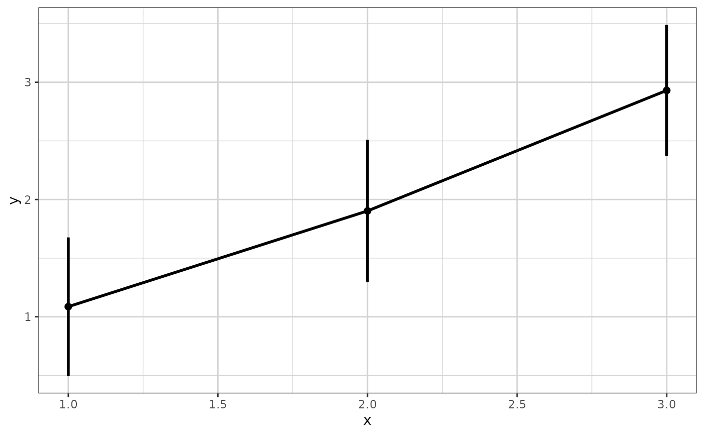
# default settings for normally distributed data, 95% confidence interval,
data <- data.frame(x = rep(c(1, 2, 3), each = 20),
y = rep(c(1, 2, 3), each = 20) + stats::rnorm(60),
group = rep(1:3, 20))
xgx_plot(data, ggplot2::aes(x = x, y = y)) +
xgx_stat_ci(conf_level = 0.95)
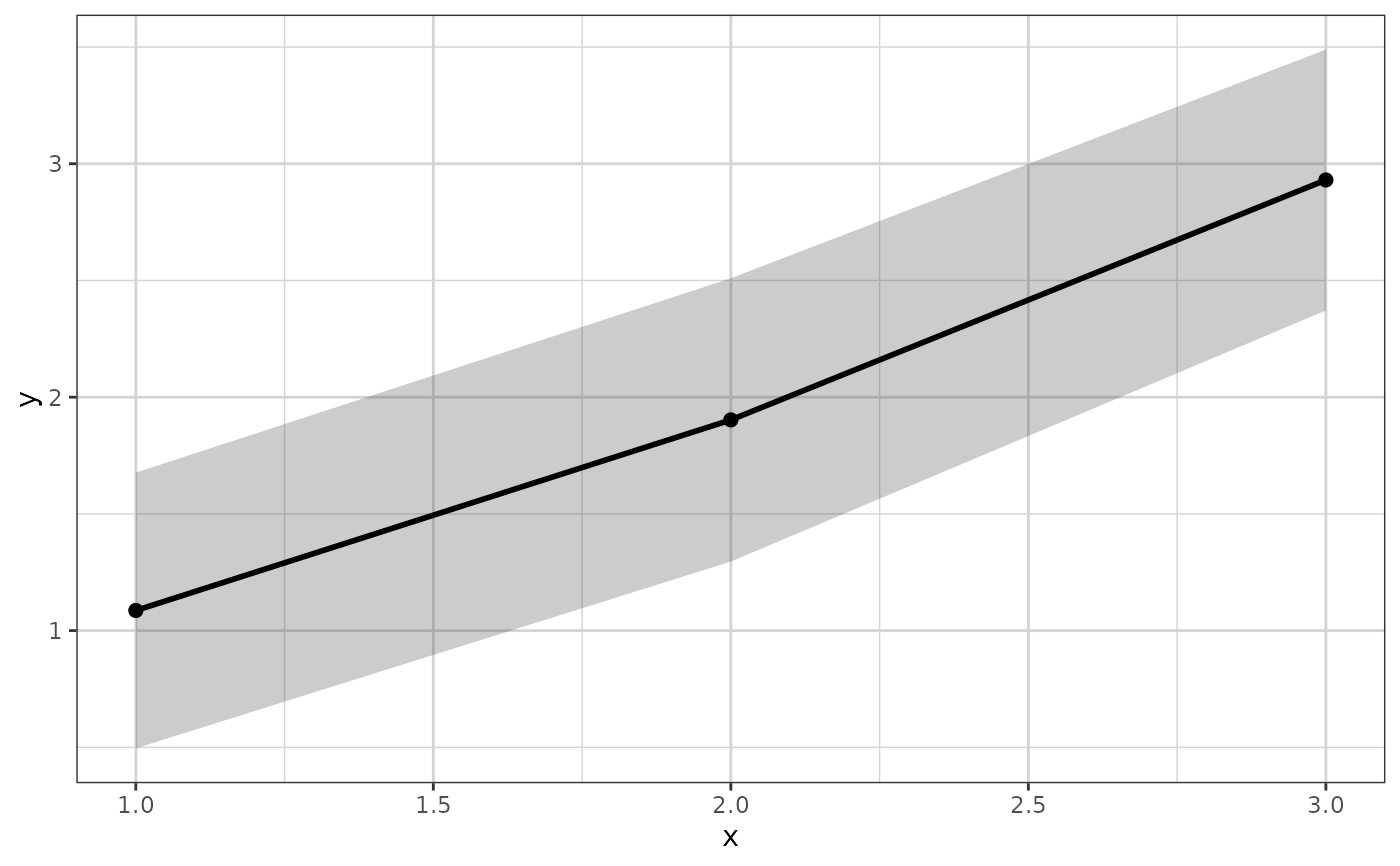
 # try different geom
xgx_plot(data, ggplot2::aes(x = x, y = y)) +
xgx_stat_ci(conf_level = 0.95, geom = list("ribbon", "point", "line"))
# try different geom
xgx_plot(data, ggplot2::aes(x = x, y = y)) +
xgx_stat_ci(conf_level = 0.95, geom = list("ribbon", "point", "line"))
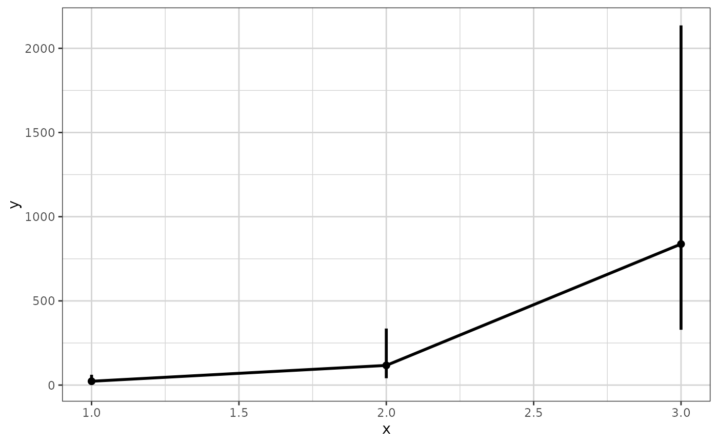
 # plotting lognormally distributed data
data <- data.frame(x = rep(c(1, 2, 3), each = 20),
y = 10^(rep(c(1, 2, 3), each = 20) + stats::rnorm(60)),
group = rep(1:3, 20))
xgx_plot(data, ggplot2::aes(x = x, y = y)) +
xgx_stat_ci(conf_level = 0.95, distribution = "lognormal")
# plotting lognormally distributed data
data <- data.frame(x = rep(c(1, 2, 3), each = 20),
y = 10^(rep(c(1, 2, 3), each = 20) + stats::rnorm(60)),
group = rep(1:3, 20))
xgx_plot(data, ggplot2::aes(x = x, y = y)) +
xgx_stat_ci(conf_level = 0.95, distribution = "lognormal")
 # note: you DO NOT need to use both distribution = "lognormal"
# and scale_y_log10()
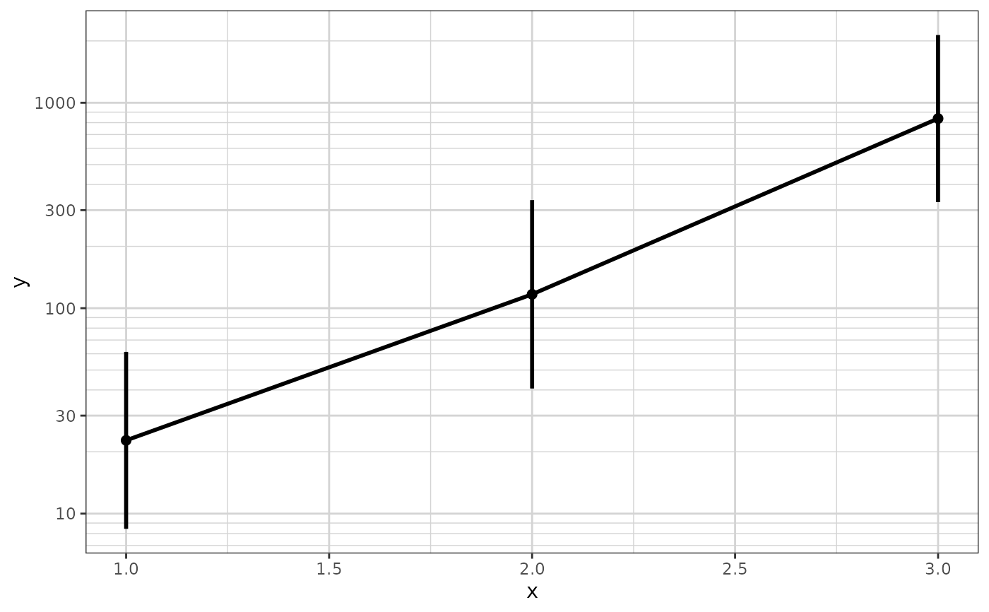
xgx_plot(data, ggplot2::aes(x = x, y = y)) +
xgx_stat_ci(conf_level = 0.95) + xgx_scale_y_log10()
# note: you DO NOT need to use both distribution = "lognormal"
# and scale_y_log10()
xgx_plot(data, ggplot2::aes(x = x, y = y)) +
xgx_stat_ci(conf_level = 0.95) + xgx_scale_y_log10()
 # plotting binomial data
data <- data.frame(x = rep(c(1, 2, 3), each = 20),
y = stats::rbinom(60, 1, rep(c(0.2, 0.6, 0.8),
each = 20)),
group = rep(1:3, 20))
xgx_plot(data, ggplot2::aes(x = x, y = y)) +
xgx_stat_ci(conf_level = 0.95, distribution = "binomial")
# plotting binomial data
data <- data.frame(x = rep(c(1, 2, 3), each = 20),
y = stats::rbinom(60, 1, rep(c(0.2, 0.6, 0.8),
each = 20)),
group = rep(1:3, 20))
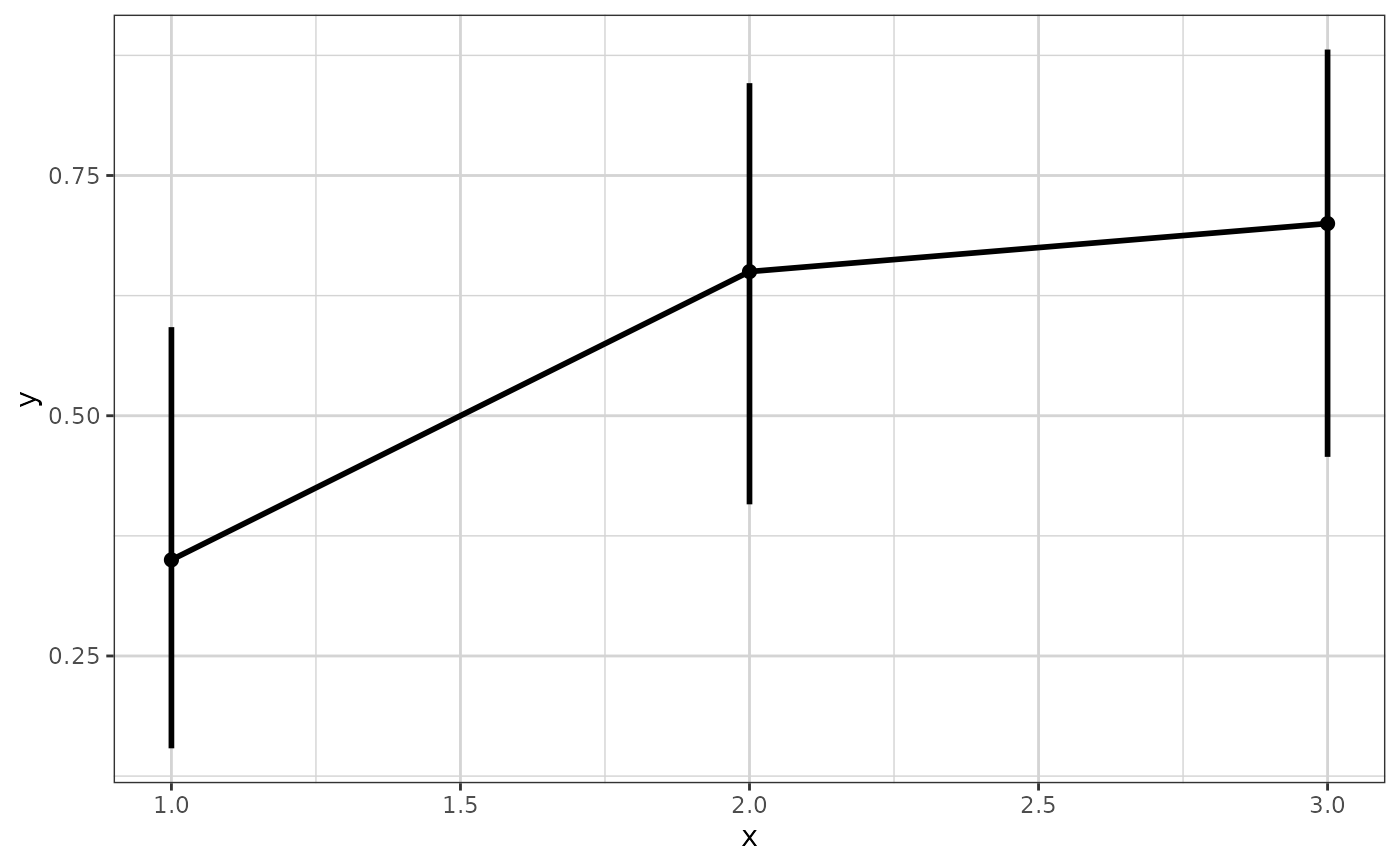
xgx_plot(data, ggplot2::aes(x = x, y = y)) +
xgx_stat_ci(conf_level = 0.95, distribution = "binomial")
 # including multiple groups in same plot
xgx_plot(data, ggplot2::aes(x = x, y = y)) +
xgx_stat_ci(conf_level = 0.95, distribution = "binomial",
ggplot2::aes(color = factor(group)),
position = ggplot2::position_dodge(width = 0.5))
# including multiple groups in same plot
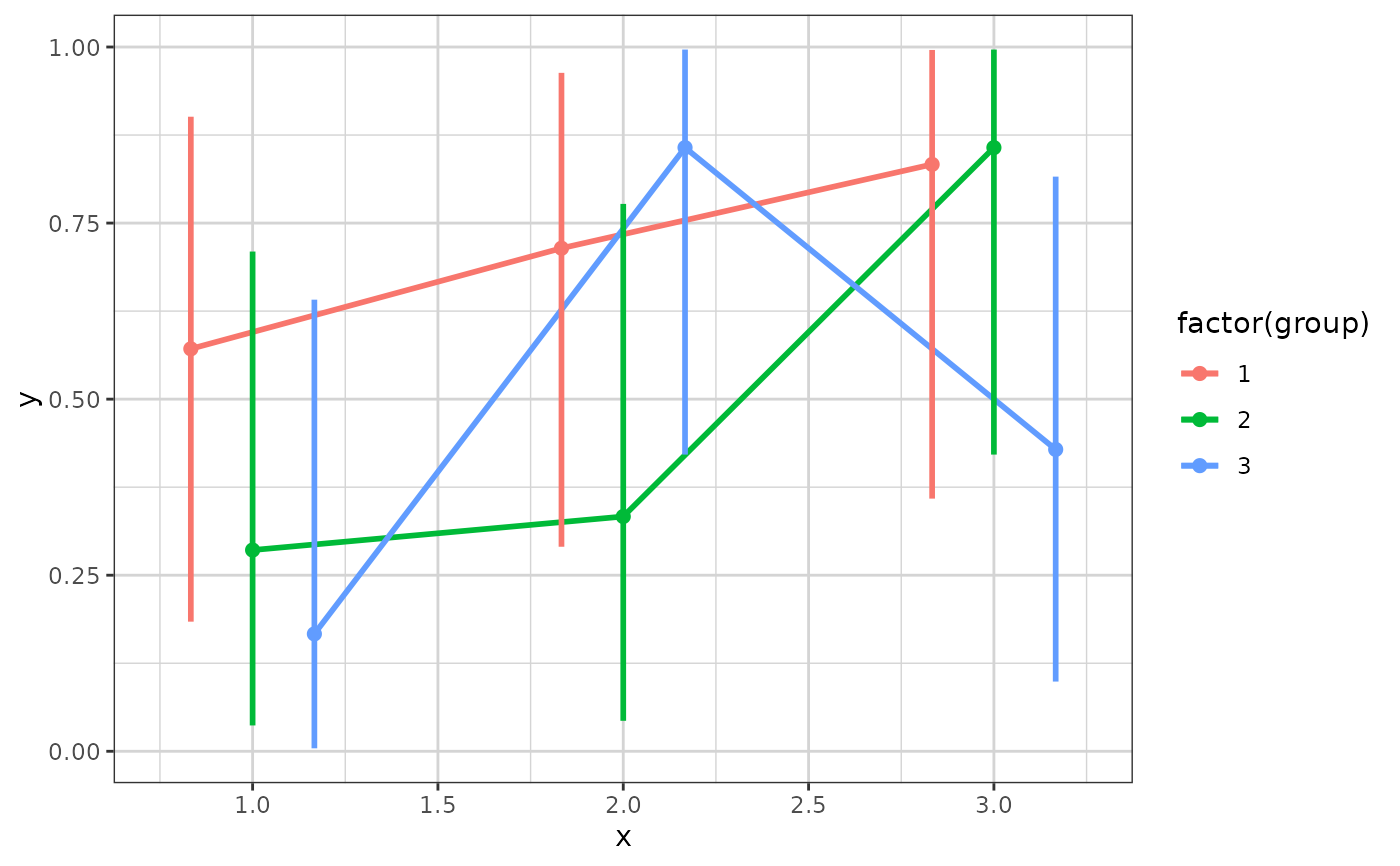
xgx_plot(data, ggplot2::aes(x = x, y = y)) +
xgx_stat_ci(conf_level = 0.95, distribution = "binomial",
ggplot2::aes(color = factor(group)),
position = ggplot2::position_dodge(width = 0.5))
 # plotting ordinal or multinomial data
set.seed(12345)
data = data.frame(x = 120*exp(stats::rnorm(100,0,1)),
response = sample(c("Mild","Moderate","Severe"), 100, replace = TRUE),
covariate = sample(c("Male","Female"), 100, replace = TRUE))
xgx_plot(data = data) +
xgx_stat_ci(mapping = ggplot2::aes(x = x, response = response, colour = covariate),
distribution = "ordinal", bins = 4) +
ggplot2::scale_y_continuous(labels = scales::percent_format()) + ggplot2::facet_wrap(~response)
#> In xgx_stat_ci:
#> The following aesthetics are identical to response: PANEL
#> These will be used for differentiating response groups in the resulting plot.
#> In xgx_stat_ci:
#> The following aesthetics are different from response: colour
#> These will be used to divide the data into different groups before calculating summary statistics on the response.
#> In xgx_stat_ci:
#> The following aesthetics are identical to response: PANEL
#> These will be used for differentiating response groups in the resulting plot.
#> In xgx_stat_ci:
#> The following aesthetics are different from response: colour
#> These will be used to divide the data into different groups before calculating summary statistics on the response.
#> In xgx_stat_ci:
#> The following aesthetics are identical to response: PANEL
#> These will be used for differentiating response groups in the resulting plot.
#> In xgx_stat_ci:
#> The following aesthetics are different from response: colour
#> These will be used to divide the data into different groups before calculating summary statistics on the response.
# plotting ordinal or multinomial data
set.seed(12345)
data = data.frame(x = 120*exp(stats::rnorm(100,0,1)),
response = sample(c("Mild","Moderate","Severe"), 100, replace = TRUE),
covariate = sample(c("Male","Female"), 100, replace = TRUE))
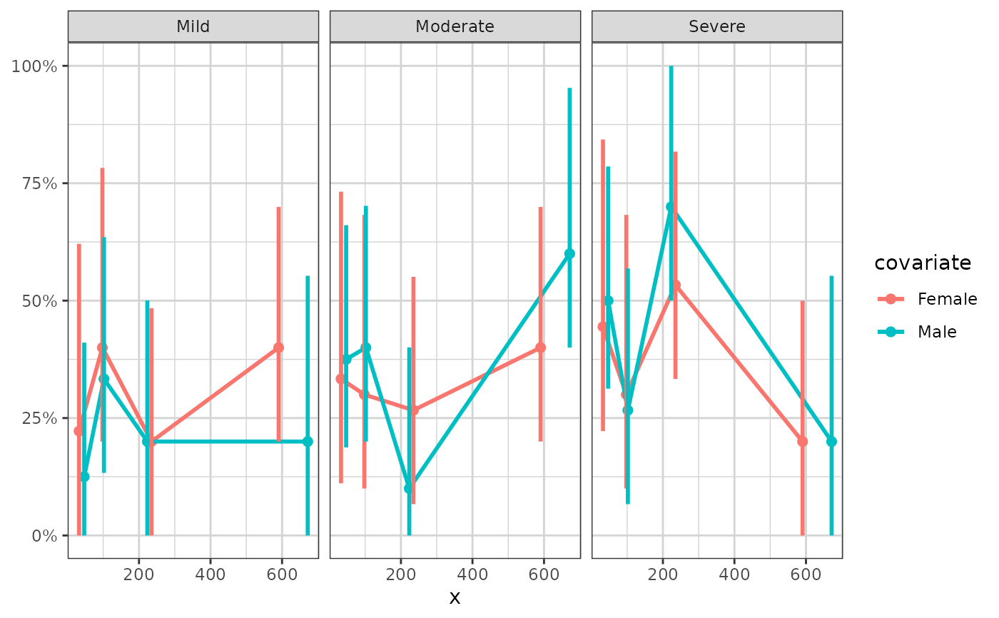
xgx_plot(data = data) +
xgx_stat_ci(mapping = ggplot2::aes(x = x, response = response, colour = covariate),
distribution = "ordinal", bins = 4) +
ggplot2::scale_y_continuous(labels = scales::percent_format()) + ggplot2::facet_wrap(~response)
#> In xgx_stat_ci:
#> The following aesthetics are identical to response: PANEL
#> These will be used for differentiating response groups in the resulting plot.
#> In xgx_stat_ci:
#> The following aesthetics are different from response: colour
#> These will be used to divide the data into different groups before calculating summary statistics on the response.
#> In xgx_stat_ci:
#> The following aesthetics are identical to response: PANEL
#> These will be used for differentiating response groups in the resulting plot.
#> In xgx_stat_ci:
#> The following aesthetics are different from response: colour
#> These will be used to divide the data into different groups before calculating summary statistics on the response.
#> In xgx_stat_ci:
#> The following aesthetics are identical to response: PANEL
#> These will be used for differentiating response groups in the resulting plot.
#> In xgx_stat_ci:
#> The following aesthetics are different from response: colour
#> These will be used to divide the data into different groups before calculating summary statistics on the response.
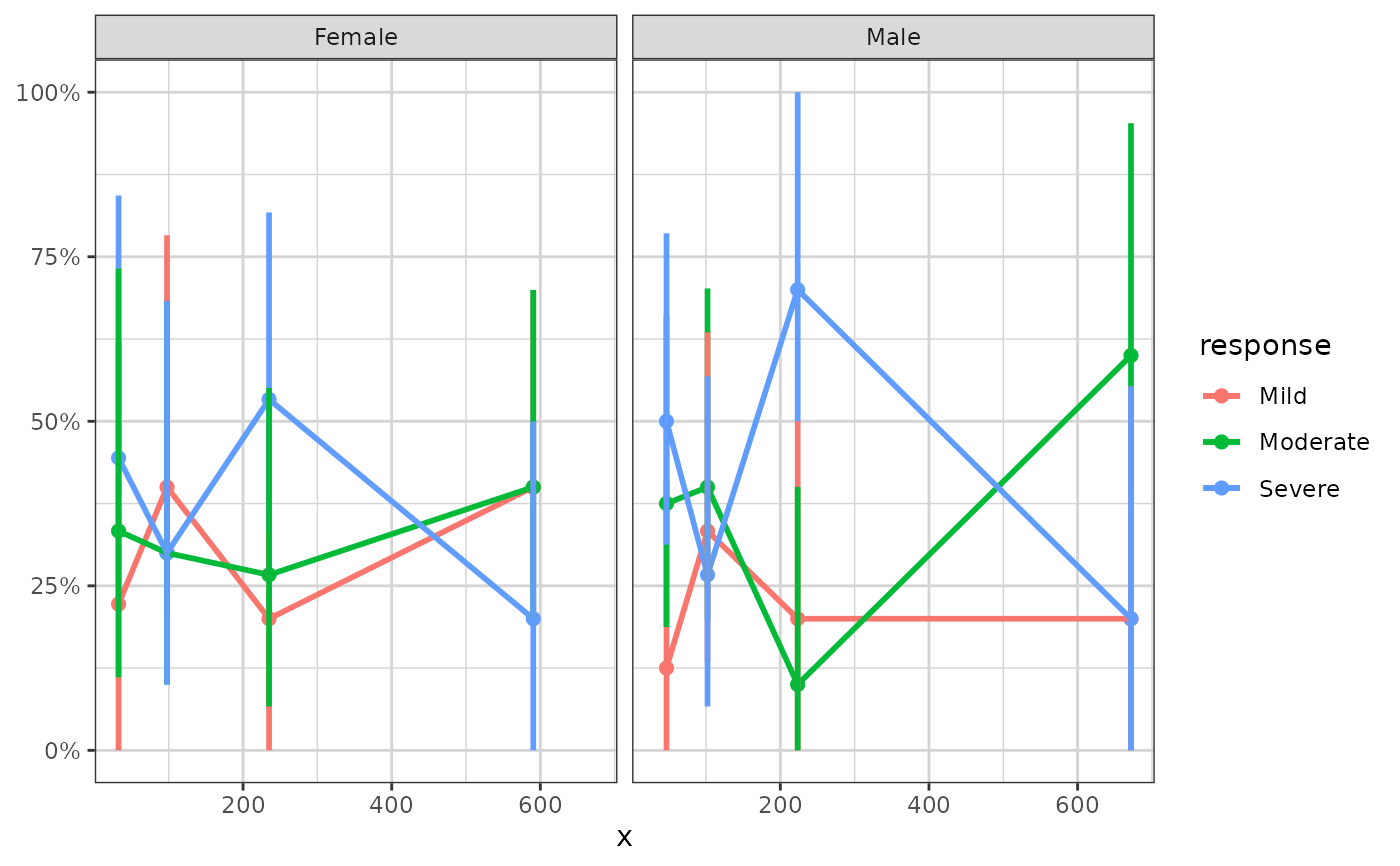
 xgx_plot(data = data) +
xgx_stat_ci(mapping = ggplot2::aes(x = x, response = response, colour = response),
distribution = "ordinal", bins = 4) +
ggplot2::scale_y_continuous(labels = scales::percent_format()) + ggplot2::facet_wrap(~covariate)
#> In xgx_stat_ci:
#> The following aesthetics are identical to response: colour
#> These will be used for differentiating response groups in the resulting plot.
#> In xgx_stat_ci:
#> The following aesthetics are different from response: PANEL
#> These will be used to divide the data into different groups before calculating summary statistics on the response.
#> In xgx_stat_ci:
#> The following aesthetics are identical to response: colour
#> These will be used for differentiating response groups in the resulting plot.
#> In xgx_stat_ci:
#> The following aesthetics are different from response: PANEL
#> These will be used to divide the data into different groups before calculating summary statistics on the response.
#> In xgx_stat_ci:
#> The following aesthetics are identical to response: colour
#> These will be used for differentiating response groups in the resulting plot.
#> In xgx_stat_ci:
#> The following aesthetics are different from response: PANEL
#> These will be used to divide the data into different groups before calculating summary statistics on the response.
xgx_plot(data = data) +
xgx_stat_ci(mapping = ggplot2::aes(x = x, response = response, colour = response),
distribution = "ordinal", bins = 4) +
ggplot2::scale_y_continuous(labels = scales::percent_format()) + ggplot2::facet_wrap(~covariate)
#> In xgx_stat_ci:
#> The following aesthetics are identical to response: colour
#> These will be used for differentiating response groups in the resulting plot.
#> In xgx_stat_ci:
#> The following aesthetics are different from response: PANEL
#> These will be used to divide the data into different groups before calculating summary statistics on the response.
#> In xgx_stat_ci:
#> The following aesthetics are identical to response: colour
#> These will be used for differentiating response groups in the resulting plot.
#> In xgx_stat_ci:
#> The following aesthetics are different from response: PANEL
#> These will be used to divide the data into different groups before calculating summary statistics on the response.
#> In xgx_stat_ci:
#> The following aesthetics are identical to response: colour
#> These will be used for differentiating response groups in the resulting plot.
#> In xgx_stat_ci:
#> The following aesthetics are different from response: PANEL
#> These will be used to divide the data into different groups before calculating summary statistics on the response.
 # Example plotting categorical vs categorical data
set.seed(12345)
data = data.frame(x = 120*exp(stats::rnorm(100,0,1)),
response = sample(c("Trt1", "Trt2", "Trt3"), 100, replace = TRUE),
covariate = factor(
sample(c("White","Black","Asian","Other"), 100, replace = TRUE),
levels = c("White", "Black", "Asian", "Other")))
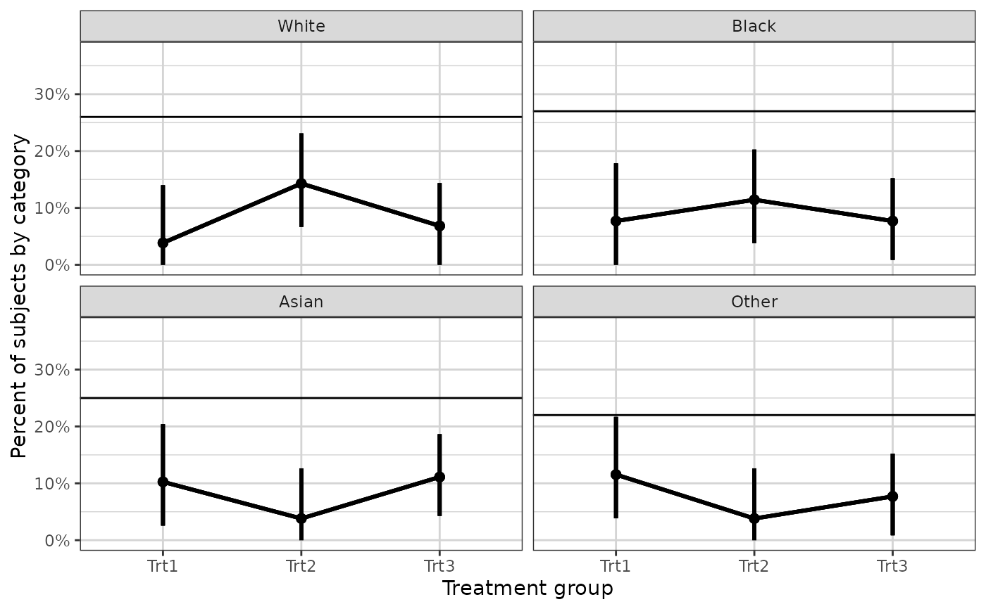
xgx_plot(data = data) +
xgx_stat_ci(mapping = ggplot2::aes(x = response, response = covariate),
distribution = "ordinal") +
xgx_stat_ci(mapping = ggplot2::aes(x = 1, response = covariate), geom = "hline",
distribution = "ordinal") +
ggplot2::scale_y_continuous(labels = scales::percent_format()) +
ggplot2::facet_wrap(~covariate) +
ggplot2::xlab("Treatment group") +
ggplot2::ylab("Percent of subjects by category")
#> In xgx_stat_ci:
#> The following aesthetics are identical to response: PANEL
#> These will be used for differentiating response groups in the resulting plot.
#> In xgx_stat_ci:
#> The following aesthetics are identical to response: PANEL
#> These will be used for differentiating response groups in the resulting plot.
#> In xgx_stat_ci:
#> The following aesthetics are identical to response: PANEL
#> These will be used for differentiating response groups in the resulting plot.
#> In xgx_stat_ci:
#> The following aesthetics are identical to response: PANEL
#> These will be used for differentiating response groups in the resulting plot.
# Example plotting categorical vs categorical data
set.seed(12345)
data = data.frame(x = 120*exp(stats::rnorm(100,0,1)),
response = sample(c("Trt1", "Trt2", "Trt3"), 100, replace = TRUE),
covariate = factor(
sample(c("White","Black","Asian","Other"), 100, replace = TRUE),
levels = c("White", "Black", "Asian", "Other")))
xgx_plot(data = data) +
xgx_stat_ci(mapping = ggplot2::aes(x = response, response = covariate),
distribution = "ordinal") +
xgx_stat_ci(mapping = ggplot2::aes(x = 1, response = covariate), geom = "hline",
distribution = "ordinal") +
ggplot2::scale_y_continuous(labels = scales::percent_format()) +
ggplot2::facet_wrap(~covariate) +
ggplot2::xlab("Treatment group") +
ggplot2::ylab("Percent of subjects by category")
#> In xgx_stat_ci:
#> The following aesthetics are identical to response: PANEL
#> These will be used for differentiating response groups in the resulting plot.
#> In xgx_stat_ci:
#> The following aesthetics are identical to response: PANEL
#> These will be used for differentiating response groups in the resulting plot.
#> In xgx_stat_ci:
#> The following aesthetics are identical to response: PANEL
#> These will be used for differentiating response groups in the resulting plot.
#> In xgx_stat_ci:
#> The following aesthetics are identical to response: PANEL
#> These will be used for differentiating response groups in the resulting plot.
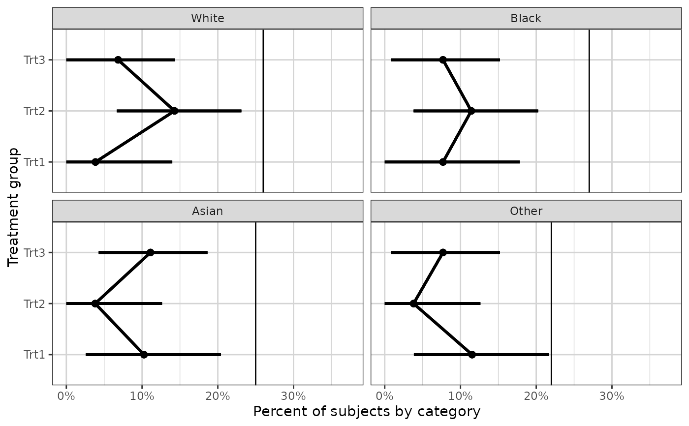
 # Same example with orientation flipped (only works for ggplot2 v.3.3.0 or later)
# only run if ggplot2 v.3.3.0 or later
ggplot2_geq_v3.3.0 <- utils::compareVersion(
as.character(utils::packageVersion("ggplot2")), '3.3.0') >= 0
if(ggplot2_geq_v3.3.0){
xgx_plot(data = data) +
xgx_stat_ci(mapping = ggplot2::aes(y = response, response = covariate), orientation = "y",
distribution = "ordinal") +
xgx_stat_ci(mapping = ggplot2::aes(y = 1, response = covariate), orientation = "y",
geom = "vline", distribution = "ordinal") +
ggplot2::scale_x_continuous(labels = scales::percent_format()) +
ggplot2::facet_wrap(~covariate) +
ggplot2::ylab("Treatment group") +
ggplot2::xlab("Percent of subjects by category")
}
#> Warning: Ignoring unknown aesthetics: y
#> In xgx_stat_ci:
#> The following aesthetics are identical to response: PANEL
#> These will be used for differentiating response groups in the resulting plot.
#> In xgx_stat_ci:
#> The following aesthetics are identical to response: PANEL
#> These will be used for differentiating response groups in the resulting plot.
#> In xgx_stat_ci:
#> The following aesthetics are identical to response: PANEL
#> These will be used for differentiating response groups in the resulting plot.
#> In xgx_stat_ci:
#> The following aesthetics are identical to response: PANEL
#> These will be used for differentiating response groups in the resulting plot.
# Same example with orientation flipped (only works for ggplot2 v.3.3.0 or later)
# only run if ggplot2 v.3.3.0 or later
ggplot2_geq_v3.3.0 <- utils::compareVersion(
as.character(utils::packageVersion("ggplot2")), '3.3.0') >= 0
if(ggplot2_geq_v3.3.0){
xgx_plot(data = data) +
xgx_stat_ci(mapping = ggplot2::aes(y = response, response = covariate), orientation = "y",
distribution = "ordinal") +
xgx_stat_ci(mapping = ggplot2::aes(y = 1, response = covariate), orientation = "y",
geom = "vline", distribution = "ordinal") +
ggplot2::scale_x_continuous(labels = scales::percent_format()) +
ggplot2::facet_wrap(~covariate) +
ggplot2::ylab("Treatment group") +
ggplot2::xlab("Percent of subjects by category")
}
#> Warning: Ignoring unknown aesthetics: y
#> In xgx_stat_ci:
#> The following aesthetics are identical to response: PANEL
#> These will be used for differentiating response groups in the resulting plot.
#> In xgx_stat_ci:
#> The following aesthetics are identical to response: PANEL
#> These will be used for differentiating response groups in the resulting plot.
#> In xgx_stat_ci:
#> The following aesthetics are identical to response: PANEL
#> These will be used for differentiating response groups in the resulting plot.
#> In xgx_stat_ci:
#> The following aesthetics are identical to response: PANEL
#> These will be used for differentiating response groups in the resulting plot.