The Alpha Release
This is an early preview of our new package, Tplyr. This package is still in development, and we’re actively working on new features. We decided to release this version early to get community feedback. If you find a bug in our code - please report it! If you’d like to see some particular feature - let us know! The more feedback we collect, the better the end product will be when we publish the first version on CRAN.
What is Tplyr?
dplyr from tidyverse is a grammar of data manipulation. So what does that allow you to do? It gives you, as a data analyst, the capability to easily and intuitively approach the problem of manipulating your data into an analysis ready form. dplyr conceptually breaks things down into verbs that allow you to focus on what you want to do more than how you have to do it.
Tplyr is designed around a similar concept, but its focus is on building summary tables within the clinical world. In the pharmaceutical industry, a great deal of the data presented in the outputs we create are very similar. For the most part, most of the tables created can be broken down into a few categories:
- Counting for event based variables or categories
- Shifting, which is just counting a ‘from’ and a ‘to’
- Generating descriptive statistics around some continuous variable.
For many of the tables that go into a clinical submission, at least when considering safety outputs, the tables are made up of a combination of these approaches. Consider a demographics table - and let’s use an example from the PHUSE project Standard Analyses & Code Sharing - Analyses & Displays Associated with Demographics, Disposition, and Medications in Phase 2-4 Clinical Trials and Integrated Summary Documents.
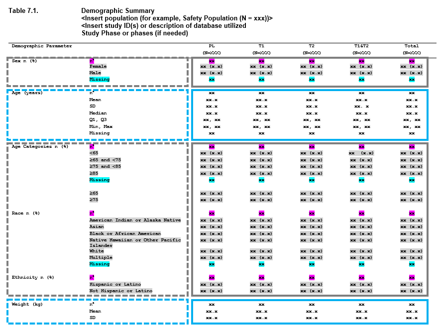
Demographics Table
When you look at this table, you can begin breaking this output down into smaller, redundant, components. These components can be viewed as ‘layers’, and the table as a whole is constructed by stacking the layers. The boxes in the image above represent how you can begin to conceptualize this.
- First we have Sex, which is made up of n (%) counts.
- Next we have Age as a continuous variable, where we have a number of descriptive statistics, including n, mean, standard deviation, median, quartile 1, quartile 3, min, max, and missing values.
- After that we have age, but broken into categories - so this is once again n (%) values.
- Race - more counting,
- Ethnicity - more counting
- Weight - and we’re back to descriptive statistics.
So we have one table, with 6 summaries (7 including the next page, not shown) - but only 2 different approaches to summaries being performed. In the same way that dplyr is a grammar of data manipulation, Tplyr aims to be a grammar of data summary. The goal of Tplyr is to allow you to program a summary table like you see it on the page, by breaking a larger problem into smaller ‘layers’, and combining them together like you see on the page.
Enough talking - let’s see some code. In these examples, we will be using data from the PHUSE Test Data Factory based on the original pilot project submission package. Note: You can see our replication of the CDISC pilot using the PHUSE Test Data Factory data here.
tplyr_table(adsl, TRT01P, where = SAFFL == "Y") %>%
  add_layer(
    group_desc(AGE, by = "Age (years)")
  ) %>%
  add_layer(
    group_count(AGEGR1, by = "Age Categories n (%)")
  ) %>%
  build()
#> # A tibble: 9 x 8
#>   row_label1 row_label2 var1_Placebo `var1_Xanomelin… `var1_Xanomelin…
#>   <chr>      <chr>      <chr>        <chr>            <chr>
#> 1 Age (year… n          " 86"        " 84"            " 84"
#> 2 Age (year… Mean (SD)  "75.2 ( 8.5… "74.4 ( 7.89)"   "75.7 ( 8.29)"
#> 3 Age (year… Median     "76.0"       "76.0"           "77.5"
#> 4 Age (year… Q1, Q3     "69.2, 81.8" "70.8, 80.0"     "71.0, 82.0"
#> 5 Age (year… Min, Max   "52, 89"     "56, 88"         "51, 88"
#> 6 Age (year… Missing    "  0"        "  0"            "  0"
#> 7 Age Categ… <65        "14 ( 16.3%… "11 ( 13.1%)"    " 8 (  9.5%)"
#> 8 Age Categ… >80        "30 ( 34.9%… "18 ( 21.4%)"    "29 ( 34.5%)"
#> 9 Age Categ… 65-80      "42 ( 48.8%… "55 ( 65.5%)"    "47 ( 56.0%)"
#> # … with 3 more variables: ord_layer_index <int>, ord_layer_1 <int>,
#> #   ord_layer_2 <dbl>
The TL;DR Before The Nitty Gritty
Here are some of the high level benefits of using Tplyr:
- Easy construction of table data using an intuitive syntax
- Smart string formatting for your numbers that’s easily specified by the user
- A great deal of flexibility in what is performed and how it’s presented, without specifying hundreds of parameters
- Extensibility (in the future…) - we’re going to open doors to allow you some level of customization.
How Tplyr Works
A Tplyr table is constructed of two main objects, a table_table object and tplyr_layer objects making up the different summaries that are to be performed.
The tplyr_table Object
The tplyr_table object is the main container upon which a tplyr table is constructed. tplyr tables are made up of one or more layers. Each layer contains an instruction for a summary to be performed. The tplyr_table object contains those layers, and the general data, metadata, and logic necessary.
When a tplyr_table is created, it will contain the following bindings:
- target - The dataset upon which summaries will be performed
- pop_data - The data containing population information. This defaults to the target dataset
- cols - A categorical variable to present summaries grouped by column (in addition to
treat_var) - table_where - The
whereparameter provided, used to subset thetargetdata - treat_var - Variable used to distinguish treatment groups.
- header_n - Default header N values based on
treat_var - pop_treat_var - The treatment variable for
pop_data(if different) - layers - The container for individual layers of a
tplyr_table - treat_grps - Additional treatment groups to be added to the summary (i.e. Total)
tplyr_table allows you a basic interface to instantiate the object. Modifier functions are available to change individual parameters catered to your analysis.
t <- tplyr_table(adsl, TRT01P, where = SAFFL == "Y")
t
#> *** tplyr_table ***
#> Target (data.frame):
#>  Name:  adsl
#>  Rows:  254
#>  Columns:  49
#> pop_data (data.frame)
#>  Name:  target
#>  Rows:  254
#>  Columns:  49
#> treat_var variable (quosure)
#>  TRT01P
#> header_n:  header groups
#> treat_grps groupings (list)
#> Table Columns (cols):
#> where: == SAFFL Y
#> Number of layer(s): 0
#> layer_output: 0
The tplyr_layer Object
Users of Tplyr interface with tplyr_layer objects using the group_<type> family of functions. This family specifies the type of summary that is to be performed within a layer. count layers are used to create summary counts of some discrete variable. desc layers create descriptive statistics, and shift layers summaries the counts of different changes in states.
-
Count Layers
- Count layers allow you to easily create summaries based on counting values with a variable. Additionally, this layer allows you to create n (%) summaries where you’re also summarizing the proportion of instances a value occurs compared to some denominator. Count layers are also capable of producing counts of nested relationships. For example, if you want to produce counts of an overall outside group, and then the subgroup counts within that group, you can simply specify the target variable as vars(OutsideVariable, InsideVariable). This allows you to do tables like Adverse Events where you want to see the Preferred Terms within Body Systems, all in one layer. NOTE: Currently, % values are calculated on the fly using header N values calculated from the target dataset. This is something that we will be adding enhanced flexibility for in future releases (remember - this is an alpha release :))
-
Descriptive Statistics Layers
- Descriptive statistics layers perform summaries on continuous variables. There are a number of summaries built into
tplyralready that you can perform, including n, mean, median, standard deviation, variance, min, max, interquartile range, Q1, Q3, and missing value counts. From these available summaries, the default presentation of a descriptive statistics layer will output ‘n’, ‘Mean (SD)’, ‘Median’, ‘Q1, Q3’, ‘Min, Max’, and ‘Missing’. You can change these summaries usingset_format_strings, and you can also add your own summaries usingset_custom_summaries. This allows you to easily implement any additional summary statistics you want presented.
- Descriptive statistics layers perform summaries on continuous variables. There are a number of summaries built into
-
Shift Layers
- NOTE: Shift layers are not yet implemented. Expect this in a future release.
cnt <- group_count(t, AGEGR1)
cnt
#> *** count_layer ***
#> Self:  count_layer < 0x55c36d686aa8 >
#> Parent:  tplyr_table < 0x55c368eec440 >
#> target_var:
#>  AGEGR1
#> by:
#> where: TRUE
#> Layer(s): 0

dsc <- group_desc(t, AGE)
dsc
#> *** desc_layer ***
#> Self:  desc_layer < 0x55c36d7e13d8 >
#> Parent:  tplyr_table < 0x55c368eec440 >
#> target_var:
#>  AGE
#> by:
#> where: TRUE
#> Layer(s): 0
Adding Layers to a Table
Everyone has their own style of coding - so we’ve tried to be flexible to an extent. Overall, tplyr is built around tidy syntax, so all of our object construction supports piping with magrittr (i.e. %>%).
There are two ways to add layers to a tplyr_table: add_layer and add_layers. The difference is that add_layer allows you to construct the layer within the call to add_layer, whereas with add_layers you can attach multiple layers that have already been constructed upfront:
t <- tplyr_table(adsl, TRT01P) %>%
  add_layer(
    group_count(AGEGR1, by = "Age categories n (%)")
  )
Within add_layer, the syntax to constructing the count layer for Age Categories was written on the fly. add_layer is special in that it also allows you to use piping to use modifier functions on the layer being constructed
t <- tplyr_table(adsl, TRT01P) %>%
  add_layer(
    group_count(AGEGR1, by = "Age categories n (%)") %>%
      set_format_strings(f_str("xx (xx.x%)", n, pct)) %>%
      add_total_row()
  )
add_layers, on the other hand, lets you isolate the code to construct a particular layer if you wanted to separate things out more. Some might find this cleaner to work with if you have a large number of layers being constructed.
t <- tplyr_table(adsl, TRT01P)

l1 <- group_count(t, AGEGR1, by = "Age categories n (%)")
l2 <- group_desc(t, AGE, by = "Age (years)")

t <- add_layers(t, l1, l2)
Notice that when you construct the layers separately, you need to specify the table to which they belong. add_layer does this automatically. tplyr_table and tplyr_layer objects are built on environments, and the parent/child relationships are very important. This is why, even though the layer knows who its table parent is, the layers still need to be attached to the table (as the table doesn’t know who its children are). Advanced R does a very good job at explaining what environments in R are, their benefits, and how to use them.
A Note Before We Go Deeper
Notice that when you construct a tplyr_table or a tplyr_layer that what displays is a summary of information about the table or layer? That’s because when you create these objects - it constructs the metadata, but does not process the actual data. This allows you to construct and make sure the pieces of your table fit together before you do the data processing - and it gives you a container to hold all of this metadata, and use it later if necessary.
To generate the data from a tplyr_table object, you use the function build:
t <- tplyr_table(adsl, TRT01P) %>%
  add_layer(
    group_count(AGEGR1, by = "Age categories n (%)")
  )

t %>% build()
#> # A tibble: 3 x 8
#>   row_label1 row_label2 var1_Placebo `var1_Xanomelin… `var1_Xanomelin…
#>   <chr>      <chr>      <chr>        <chr>            <chr>
#> 1 Age categ… <65        14 ( 16.3%)  11 ( 13.1%)      " 8 (  9.5%)"
#> 2 Age categ… >80        30 ( 34.9%)  18 ( 21.4%)      "29 ( 34.5%)"
#> 3 Age categ… 65-80      42 ( 48.8%)  55 ( 65.5%)      "47 ( 56.0%)"
#> # … with 3 more variables: ord_layer_index <int>, ord_layer_1 <int>,
#> #   ord_layer_2 <dbl>
But there’s more you can get from Tplyr. It’s great to have the formatted numbers, but what about the numeric data behind the scenes? What if you want to calculate your own statistics based off of the counts? You can get that information as well using get_numeric_data. This returns the numeric data from each layer as a list of data frames:
get_numeric_data(t)
#> [[1]]
#> # A tibble: 9 x 5
#>   TRT01P               `"Age categories n (%)"` summary_var     n total
#>   <chr>                <chr>                    <chr>       <dbl> <int>
#> 1 Placebo              Age categories n (%)     <65            14    86
#> 2 Placebo              Age categories n (%)     >80            30    86
#> 3 Placebo              Age categories n (%)     65-80          42    86
#> 4 Xanomeline High Dose Age categories n (%)     <65            11    84
#> 5 Xanomeline High Dose Age categories n (%)     >80            18    84
#> 6 Xanomeline High Dose Age categories n (%)     65-80          55    84
#> 7 Xanomeline Low Dose  Age categories n (%)     <65             8    84
#> 8 Xanomeline Low Dose  Age categories n (%)     >80            29    84
#> 9 Xanomeline Low Dose  Age categories n (%)     65-80          47    84
By storing pertinent information, you can get more out of a Tplyr objects than processed data for display. And by specifying when you want to get data out of Tplyr, we can save you from repeatedly processing data while your constructing your outputs - which is particularly useful when that computation starts taking time.
Constructing Layers
The bulk of Tplyr coding comes from constructing your layers and specifying the work you want to be done. Before we get into this, it’s important to discuss how Tplyr handles string formatting.
String Formatting in Tplyr
String formatting in Tplyr is controlled by an object called an f_str, which is also the name of function you use to create these formats. To set these format strings into a tplyr_layer, you use the function set_format_strings, and this usage varies slightly between layer types (more on that later).
So - why is this object necessary. Consider this example:
t <- tplyr_table(adsl, TRT01P) %>%
  add_layer(
    group_desc(AGE, by = "Age (years)") %>%
      set_format_strings(
        'n' = f_str('xx', n),
        'Mean (SD)' = f_str('xx.xx (xx.xxx)', mean, sd)
      )
  )

t %>% build()
#> # A tibble: 2 x 8
#>   row_label1 row_label2 var1_Placebo `var1_Xanomelin… `var1_Xanomelin…
#>   <chr>      <chr>      <chr>        <chr>            <chr>
#> 1 Age (year… n          86           84               84
#> 2 Age (year… Mean (SD)  75.21 ( 8.5… 74.38 ( 7.886)   75.67 ( 8.286)
#> # … with 3 more variables: ord_layer_index <int>, ord_layer_1 <int>,
#> #   ord_layer_2 <int>
In a perfect world, the f_str calls wouldn’t be necessary - but in reality they allow us to infer a great deal of information from realistically very few user inputs. In the calls that you see above:
- The row labels in the
row_label2column are taken from the left side of each=inset_format_strings - The string formats, including integer length and decimal precision, and exact presentation formatting are taken from the strings within the first parameter of each
f_strcall - The second and greater parameters within each f_str call determine the descriptive statistic summaries that will be performed. This is connected to a number of default summaries available within
Tplyr, but you can also create your own summaries (more on that later). The default summaries that are built in include:-
n= Number of observations -
mean= Mean -
sd= Standard Deviation -
var= Variance -
iqr= Inter Quartile Range -
q1= 1st quartile -
q3= 3rd quartile -
min= Minimum value -
max= Maximum value -
missing= Count of NA values
-
- When two summaries are placed on the same
f_strcall, then those two summaries are formatted into the same string. This allows you to do aMean (SD)type format where both numbers appear.
This simple user input controls a significant amount of work in the back end of the data processing, and the f_str object allows that metadata to be collected.
f_str objects are also used with count layers as well to control the data presentation. Instead of specifying the summaries performed, you use n and pct for your parameters, if you want both n’s and percents presented.
tplyr_table(adsl, TRT01P) %>%
  add_layer(
    group_count(AGEGR1, by = "Age categories") %>%
      set_format_strings(f_str('xx (xx.x)',n,pct))
  ) %>%
  build()
#> # A tibble: 3 x 8
#>   row_label1 row_label2 var1_Placebo `var1_Xanomelin… `var1_Xanomelin…
#>   <chr>      <chr>      <chr>        <chr>            <chr>
#> 1 Age categ… <65        14 (16.3)    11 (13.1)        " 8 ( 9.5)"
#> 2 Age categ… >80        30 (34.9)    18 (21.4)        "29 (34.5)"
#> 3 Age categ… 65-80      42 (48.8)    55 (65.5)        "47 (56.0)"
#> # … with 3 more variables: ord_layer_index <int>, ord_layer_1 <int>,
#> #   ord_layer_2 <dbl>

tplyr_table(adsl, TRT01P) %>%
  add_layer(
    group_count(AGEGR1, by = "Age categories") %>%
      set_format_strings(f_str('xx',n))
  ) %>%
  build()
#> # A tibble: 3 x 8
#>   row_label1 row_label2 var1_Placebo `var1_Xanomelin… `var1_Xanomelin…
#>   <chr>      <chr>      <chr>        <chr>            <chr>
#> 1 Age categ… <65        14           11               " 8"
#> 2 Age categ… >80        30           18               "29"
#> 3 Age categ… 65-80      42           55               "47"
#> # … with 3 more variables: ord_layer_index <int>, ord_layer_1 <int>,
#> #   ord_layer_2 <dbl>
Really - format strings allow you to present your data however you like.
tplyr_table(adsl, TRT01P) %>%
  add_layer(
    group_count(AGEGR1, by = "Age categories") %>%
      set_format_strings(f_str('xx (•◡•) xx.x%',n,pct))
  ) %>%
  build()
#> # A tibble: 3 x 8
#>   row_label1 row_label2 var1_Placebo `var1_Xanomelin… `var1_Xanomelin…
#>   <chr>      <chr>      <chr>        <chr>            <chr>
#> 1 Age categ… <65        14 (•◡•) 16… 11 (•◡•) 13.1%   " 8 (•◡•)  9.5%"
#> 2 Age categ… >80        30 (•◡•) 34… 18 (•◡•) 21.4%   "29 (•◡•) 34.5%"
#> 3 Age categ… 65-80      42 (•◡•) 48… 55 (•◡•) 65.5%   "47 (•◡•) 56.0%"
#> # … with 3 more variables: ord_layer_index <int>, ord_layer_1 <int>,
#> #   ord_layer_2 <dbl>
But should you? Probably not.
Descriptive Statistic Layers
As covered under string formatting, set_format_strings controls a great deal of what happens within a descriptive statistics layer. Note that there are some built in defaults to what’s output:
tplyr_table(adsl, TRT01P) %>%
  add_layer(
    group_desc(AGE, by = "Age (years)")
  ) %>%
  build()
#> # A tibble: 6 x 8
#>   row_label1 row_label2 var1_Placebo `var1_Xanomelin… `var1_Xanomelin…
#>   <chr>      <chr>      <chr>        <chr>            <chr>
#> 1 Age (year… n          " 86"        " 84"            " 84"
#> 2 Age (year… Mean (SD)  "75.2 ( 8.5… "74.4 ( 7.89)"   "75.7 ( 8.29)"
#> 3 Age (year… Median     "76.0"       "76.0"           "77.5"
#> 4 Age (year… Q1, Q3     "69.2, 81.8" "70.8, 80.0"     "71.0, 82.0"
#> 5 Age (year… Min, Max   "52, 89"     "56, 88"         "51, 88"
#> 6 Age (year… Missing    "  0"        "  0"            "  0"
#> # … with 3 more variables: ord_layer_index <int>, ord_layer_1 <int>,
#> #   ord_layer_2 <int>
To override these defaults, just specify the summaries that you want to be performed using set_format_strings as described above. But what if Tplyr doesn’t have a built in function to do the summary statistic that you want to see? Well - you can make your own! This is where set_custom_summaries comes into play. Let’s say you want to derive a geometric mean.
tplyr_table(adsl, TRT01P) %>%
  add_layer(
    group_desc(AGE, by = "Sepal Length") %>%
      set_custom_summaries(
        geometric_mean = exp(sum(log(.var[.var > 0]), na.rm=TRUE) / length(.var))
      ) %>%
      set_format_strings(
        'Geometric Mean (SD)' = f_str('xx.xx (xx.xxx)', geometric_mean, sd)
      )
  ) %>%
  build()
#> # A tibble: 1 x 8
#>   row_label1 row_label2 var1_Placebo `var1_Xanomelin… `var1_Xanomelin…
#>   <chr>      <chr>      <chr>        <chr>            <chr>
#> 1 Sepal Len… Geometric… 74.70 ( 8.5… 73.94 ( 7.886)   75.18 ( 8.286)
#> # … with 3 more variables: ord_layer_index <int>, ord_layer_1 <int>,
#> #   ord_layer_2 <int>
In set_custom_summaries, first you name the summary being performed. This is important - that name is what you use in the f_str call to incorporate it into a format. Next, you program or call the function desired. What happens in the background is that this is used in a call to dplyr::summarize - so use similar syntax. Use the variable name .var in your custom summary function. This is necessary because it allows a generic variable name to be used when multiple target variables are specified - and therefore the function can be applied to both target variables.
Sometimes there’s a need to present multiple variables summarized side by side. Tplyr makes this easy as well.
tplyr_table(adsl, TRT01P) %>%
  add_layer(
    group_desc(vars(AGE, AVGDD), by = "Age and Avg. Daily Dose")
  ) %>%
  build()
#> # A tibble: 6 x 11
#>   row_label1 row_label2 var1_Placebo `var1_Xanomelin… `var1_Xanomelin…
#>   <chr>      <chr>      <chr>        <chr>            <chr>
#> 1 Age and A… n          " 86"        " 84"            " 84"
#> 2 Age and A… Mean (SD)  "75.2 ( 8.5… "74.4 ( 7.89)"   "75.7 ( 8.29)"
#> 3 Age and A… Median     "76.0"       "76.0"           "77.5"
#> 4 Age and A… Q1, Q3     "69.2, 81.8" "70.8, 80.0"     "71.0, 82.0"
#> 5 Age and A… Min, Max   "52, 89"     "56, 88"         "51, 88"
#> 6 Age and A… Missing    "  0"        "  0"            "  0"
#> # … with 6 more variables: var2_Placebo <chr>, `var2_Xanomeline High
#> #   Dose` <chr>, `var2_Xanomeline Low Dose` <chr>, ord_layer_index <int>,
#> #   ord_layer_1 <int>, ord_layer_2 <int>
Tplyr summarizes both variables and merges them together. This makes creating tables where you need to compare BASE, AVAL, and CHG next to each other nice and simple. Note the use of vars - in any situation where you’d like to use multiple variable names in a parameter, use dplyr::vars to specify the variables. You can use text strings in the calls to dplyr::vars as well.
Count Layers
Count layers generally allow you to create n and n (%) count type summaries. There are a few extra features here as well. Let’s say that you want a total row within your counts. This is easy with add_total_row():
tplyr_table(adsl, TRT01P) %>%
  add_layer(
    group_count(AGEGR1, by = "Age categories") %>%
      add_total_row()
  ) %>%
  build()
#> # A tibble: 4 x 8
#>   row_label1 row_label2 var1_Placebo `var1_Xanomelin… `var1_Xanomelin…
#>   <chr>      <chr>      <chr>        <chr>            <chr>
#> 1 Age categ… <65        14 ( 16.3%)  11 ( 13.1%)      " 8 (  9.5%)"
#> 2 Age categ… >80        30 ( 34.9%)  18 ( 21.4%)      "29 ( 34.5%)"
#> 3 Age categ… 65-80      42 ( 48.8%)  55 ( 65.5%)      "47 ( 56.0%)"
#> 4 Age categ… NA         86 (100.0%)  84 (100.0%)      "84 (100.0%)"
#> # … with 3 more variables: ord_layer_index <int>, ord_layer_1 <int>,
#> #   ord_layer_2 <dbl>
Sometimes it’s also necessary to count summaries based on distinct values. Tplyr allows you to do this as well with set_distinct_by:
tplyr_table(adae, TRTA) %>%
  add_layer(
    group_count('Subjects with at least one adverse event') %>%
      set_distinct_by(USUBJID) %>%
      set_format_strings(f_str('xx', n))
  ) %>%
  build()
#> # A tibble: 1 x 6
#>   row_label1 var1_Placebo `var1_Xanomelin… `var1_Xanomelin… ord_layer_index
#>   <chr>      <chr>        <chr>            <chr>                      <int>
#> 1 Subjects … " 47"        111              118                            1
#> # … with 1 more variable: ord_layer_1 <lgl>
There’s another trick going on here - to create a summary with row label text like you see above, text strings can be used as the target variables. Here, we use this in combination with set_distinct_by to count distinct subjects.
Adverse event tables often call for counting AEs of something like a body system and counting actual events within that body system. Tplyr has means of making this simple for the user as well.
tplyr_table(adae, TRTA) %>%
  add_layer(
    group_count(vars(AEBODSYS, AEDECOD))
  ) %>%
  build()
#> # A tibble: 22 x 8
#>    row_label1 row_label2 var1_Placebo `var1_Xanomelin… `var1_Xanomelin…
#>    <chr>      <chr>      <chr>        <chr>            <chr>
#>  1 SKIN AND … "SKIN AND… " 47 (100.0… "111 (100.0%)"   "118 (100.0%)"
#>  2 SKIN AND … "   ACTIN… "  0 (  0.0… "  1 (  0.9%)"   "  0 (  0.0%)"
#>  3 SKIN AND … "   ALOPE… "  1 (  2.1… "  0 (  0.0%)"   "  0 (  0.0%)"
#>  4 SKIN AND … "   BLIST… "  0 (  0.0… "  2 (  1.8%)"   "  8 (  6.8%)"
#>  5 SKIN AND … "   COLD … "  3 (  6.4… "  0 (  0.0%)"   "  0 (  0.0%)"
#>  6 SKIN AND … "   DERMA… "  1 (  2.1… "  0 (  0.0%)"   "  0 (  0.0%)"
#>  7 SKIN AND … "   DERMA… "  0 (  0.0… "  0 (  0.0%)"   "  2 (  1.7%)"
#>  8 SKIN AND … "   DRUG … "  1 (  2.1… "  0 (  0.0%)"   "  0 (  0.0%)"
#>  9 SKIN AND … "   ERYTH… " 13 ( 27.7… " 22 ( 19.8%)"   " 24 ( 20.3%)"
#> 10 SKIN AND … "   HYPER… "  2 (  4.3… " 10 (  9.0%)"   "  5 (  4.2%)"
#> # … with 12 more rows, and 3 more variables: ord_layer_index <int>,
#> #   ord_layer_1 <int>, ord_layer_2 <dbl>
Note that the nesting of variables happens automatically.
Other Bells and Whistles
For simplicity of demonstration, some other features have not yet been demonstrated - so let’s get into that now!
First up, it’s common to have to present a total group, or a treated group vs. the placebo. Tplyr allows you to create these groups as necessary using add_treat_group and the abbreviated function add_total_group.
tplyr_table(adsl, TRT01P) %>%
  add_total_group() %>%
  add_treat_grps(Treated = c("Xanomeline High Dose", "Xanomeline Low Dose")) %>%
  add_layer(
    group_count(AGEGR1, by = "Age categories")
  ) %>%
  build()
#> # A tibble: 3 x 10
#>   row_label1 row_label2 var1_Placebo var1_Total var1_Treated `var1_Xanomelin…
#>   <chr>      <chr>      <chr>        <chr>      <chr>        <chr>
#> 1 Age categ… <65        " 14 ( 16.3… " 33 ( 13… " 19 ( 11.3… " 11 ( 13.1%)"
#> 2 Age categ… >80        " 30 ( 34.9… " 77 ( 30… " 47 ( 28.0… " 18 ( 21.4%)"
#> 3 Age categ… 65-80      " 42 ( 48.8… "144 ( 56… "102 ( 60.7… " 55 ( 65.5%)"
#> # … with 4 more variables: `var1_Xanomeline Low Dose` <chr>,
#> #   ord_layer_index <int>, ord_layer_1 <int>, ord_layer_2 <dbl>
What about having different by group variables? So far I’ve only demonstrated by to present row label text. It additionally allows you to use grouping variables as well:
tplyr_table(adsl, TRT01P) %>%
  add_layer(
    group_count(AGEGR1, by = vars("Age categories", SEX))
  ) %>%
  build()
#> # A tibble: 6 x 10
#>   row_label1 row_label2 row_label3 var1_Placebo `var1_Xanomelin…
#>   <chr>      <chr>      <chr>      <chr>        <chr>
#> 1 Age categ… F          <65        " 9 ( 10.5%… " 5 (  6.0%)"
#> 2 Age categ… F          >80        "22 ( 25.6%… " 7 (  8.3%)"
#> 3 Age categ… F          65-80      "22 ( 25.6%… "28 ( 33.3%)"
#> 4 Age categ… M          <65        " 5 (  5.8%… " 6 (  7.1%)"
#> 5 Age categ… M          >80        " 8 (  9.3%… "11 ( 13.1%)"
#> 6 Age categ… M          65-80      "20 ( 23.3%… "27 ( 32.1%)"
#> # … with 5 more variables: `var1_Xanomeline Low Dose` <chr>,
#> #   ord_layer_index <int>, ord_layer_1 <int>, ord_layer_2 <int>,
#> #   ord_layer_3 <dbl>
Grouping by columns? We’ve got that to - but this is actually specified at the tplyr_table level. Why? It gets complicated if layers don’t have consistent columns, and stacking them together would get complex. Similarly, assuming you’d want the cols argument the same between layers, it’s more tedious to specify it on every layer constructor.
tplyr_table(adsl, TRT01P, cols=SEX) %>%
  add_layer(
    group_count(AGEGR1, by = "Age categories")
  ) %>%
  build()
#> # A tibble: 3 x 11
#>   row_label1 row_label2 var1_Placebo_F var1_Placebo_M `var1_Xanomelin…
#>   <chr>      <chr>      <chr>          <chr>          <chr>
#> 1 Age categ… <65        " 9 ( 17.0%)"  " 5 ( 15.2%)"  " 5 ( 12.5%)"
#> 2 Age categ… >80        "22 ( 41.5%)"  " 8 ( 24.2%)"  " 7 ( 17.5%)"
#> 3 Age categ… 65-80      "22 ( 41.5%)"  "20 ( 60.6%)"  "28 ( 70.0%)"
#> # … with 6 more variables: `var1_Xanomeline High Dose_M` <chr>,
#> #   `var1_Xanomeline Low Dose_F` <chr>, `var1_Xanomeline Low Dose_M` <chr>,
#> #   ord_layer_index <int>, ord_layer_1 <int>, ord_layer_2 <dbl>
Note that in both by and cols - multiple variable names (or text along with variable names) should be specified using dplyr::vars. We’ve tried to make the error messages explicit when you fail to do this, and help remind you of the proper parameter entry.
Preparing Your Table for Presentation
Now that we’ve gotten through a lot of the functionality of Tplyr, what about when you’re ready to present your table? Well - we’re deferring the cosmetics to packages that already do this exceptionally well. We’re big fans of huxtable, as you may have seen from our package pharmaRTF. RStudio is continually working on and improving gt - so we’re not reinventing the wheel here. But we can do our part to make it easier.
In a huxtable - the column headers of a table are just rows in a table. To make this preperation easier, we made the function add_column_headers into Tplyr. This allows you to simply use a string to created column headers - and it supports nesting. Let’s see it in action.
tplyr_table(adsl, TRT01P) %>%
  add_layer(
    group_desc(AGE, by = "Age (Years)")
  ) %>%
  build() %>%
  mutate_all(as.character) %>%
  add_column_headers(
    ' | Statistic | Placebo | Xanomeline (High) | Xanomeline (Low) | ord_layer_index | ord_layer_1 | ord_layer_2'
  )
#> # A tibble: 7 x 8
#>   row_label1 row_label2 var1_Placebo `var1_Xanomelin… `var1_Xanomelin…
#>   <chr>      <chr>      <chr>        <chr>            <chr>
#> 1 ""         Statistic  "Placebo"    "Xanomeline (Hi… "Xanomeline (Lo…
#> 2 "Age (Yea… n          " 86"        " 84"            " 84"
#> 3 "Age (Yea… Mean (SD)  "75.2 ( 8.5… "74.4 ( 7.89)"   "75.7 ( 8.29)"
#> 4 "Age (Yea… Median     "76.0"       "76.0"           "77.5"
#> 5 "Age (Yea… Q1, Q3     "69.2, 81.8" "70.8, 80.0"     "71.0, 82.0"
#> 6 "Age (Yea… Min, Max   "52, 89"     "56, 88"         "51, 88"
#> 7 "Age (Yea… Missing    "  0"        "  0"            "  0"
#> # … with 3 more variables: ord_layer_index <chr>, ord_layer_1 <chr>,
#> #   ord_layer_2 <chr>
Columns are separated with the bar character (|). Nesting is done by adding text in curly brackets (i.e. {}).
tplyr_table(adsl, TRT01P) %>%
  add_layer(
    group_desc(vars(AGE, AVGDD), by = "Age and Avg. Daily Dose")
  ) %>%
  build() %>%
  mutate_all(as.character) %>%
  add_column_headers(
    ' | Statistic | Age {Placebo | Xanomeline (High) | Xanomeline (Low)} | Average Daily Dose {Placebo | Xanomeline (High) | Xanomeline (Low)} | Layer Index | Layer Order 1 | Layer Order 2'
  )
#> # A tibble: 8 x 11
#>   row_label1 row_label2 var1_Placebo `var1_Xanomelin… `var1_Xanomelin…
#>   <chr>      <chr>      <chr>        <chr>            <chr>
#> 1 ""         ""         "Age"        ""               ""
#> 2 ""         "Statisti… "Placebo"    "Xanomeline (Hi… "Xanomeline (Lo…
#> 3 "Age and … "n"        " 86"        " 84"            " 84"
#> 4 "Age and … "Mean (SD… "75.2 ( 8.5… "74.4 ( 7.89)"   "75.7 ( 8.29)"
#> 5 "Age and … "Median"   "76.0"       "76.0"           "77.5"
#> 6 "Age and … "Q1, Q3"   "69.2, 81.8" "70.8, 80.0"     "71.0, 82.0"
#> 7 "Age and … "Min, Max" "52, 89"     "56, 88"         "51, 88"
#> 8 "Age and … "Missing"  "  0"        "  0"            "  0"
#> # … with 6 more variables: var2_Placebo <chr>, `var2_Xanomeline High
#> #   Dose` <chr>, `var2_Xanomeline Low Dose` <chr>, ord_layer_index <chr>,
#> #   ord_layer_1 <chr>, ord_layer_2 <chr>
Tying It All Together
Ok - so, this was a lot to cover. But how does this all fit in the grand scheme of things? Let’s look at a more complete example - what if we wanted to build that demographics table
t <- tplyr_table(adsl, TRT01P, where = (SAFFL == "Y")) %>%
  add_total_group() %>%
  add_layer(
    group_count(SEX, by="Sex") %>%
      set_format_strings(f_str("xx (xxx%)",n,pct))
  ) %>%
  add_layer(
    group_desc(AGE, by="Age Categories")
  ) %>%
  add_layer(
    group_count(RACE, by="Race") %>%
      set_format_strings(f_str("xx (xxx%)",n,pct))
  ) %>%
  add_layer(
    group_count(ETHNIC, by="Ethnicity") %>%
      set_format_strings(f_str("xx (xxx%)",n,pct))
  ) %>%
  add_layer(
    group_desc(WEIGHTBL, by="Weight")
  )

# build the table
t %>%
  build() %>%
  select(starts_with('row_label'), var1_Placebo, starts_with('var1_X'), var1_Total) %>%
  add_column_headers(" |  | Placebo | Xanomeline (Low) | Xanomeline (High) | Total") %>%
  apply_row_masks() %>%
  huxtable::as_hux(add_colnames=FALSE)
| Placebo | Xanomeline (Low) | Xanomeline (High) | Total | ||
| Sex | F | 53 ( 62%) | 40 ( 48%) | 50 ( 60%) | 143 ( 56%) |
| M | 33 ( 38%) | 44 ( 52%) | 34 ( 40%) | 111 ( 44%) | |
| Age Categories | n | 86 | 84 | 84 | 254 |
| Mean (SD) | 75.2 ( 8.59) | 74.4 ( 7.89) | 75.7 ( 8.29) | 75.1 ( 8.25) | |
| Median | 76.0 | 76.0 | 77.5 | 77.0 | |
| Q1, Q3 | 69.2, 81.8 | 70.8, 80.0 | 71.0, 82.0 | 70.0, 81.0 | |
| Min, Max | 52, 89 | 56, 88 | 51, 88 | 51, 89 | |
| Missing | 0 | 0 | 0 | 0 | |
| Race | AMERICAN INDIAN OR ALASKA NATIVE | 0 ( 0%) | 1 ( 1%) | 0 ( 0%) | 1 ( 0%) |
| BLACK OR AFRICAN AMERICAN | 8 ( 9%) | 9 ( 11%) | 6 ( 7%) | 23 ( 9%) | |
| WHITE | 78 ( 91%) | 74 ( 88%) | 78 ( 93%) | 230 ( 91%) | |
| Ethnicity | HISPANIC OR LATINO | 3 ( 3%) | 3 ( 4%) | 6 ( 7%) | 12 ( 5%) |
| NOT HISPANIC OR LATINO | 83 ( 97%) | 81 ( 96%) | 78 ( 93%) | 242 ( 95%) | |
| Weight | n | 86 | 84 | 84 | 254 |
| Mean (SD) | 62.76 ( 12.772) | 70.00 ( 14.653) | 67.28 ( 14.124) | 66.65 ( 14.131) | |
| Median | 60.55 | 69.20 | 64.90 | 66.70 | |
| Q1, Q3 | 53.62, 74.18 | 56.98, 80.30 | 56.05, 77.45 | 55.30, 77.10 | |
| Min, Max | 34.0, 86.2 | 41.7, 108.0 | 45.4, 106.1 | 34.0, 108.0 | |
| Missing | 0 | 0 | 1 | 1 |
And just like that - you have a huxtable table ready to go.
Wouldn’t it be nice if you had some resources for where to take it from here? Oh wait - you do! This is the perfect point to take things to the next step in the workflow: preparing and delivering your final output. We have plenty for you to read in our pharmaRTF vignettes about how to get started with huxtable, and create your RTF output files.
This is the alpha release - what’s next?
We’ve gotten a lot built into Tplyr, but there’s a ways to go. Here are some of the things that we’re planning to implement but don’t have ready yet:
- Modifying denominators used in counts. They’re currently calculated based on treatment group on the fly. There are a lot of ways to do this, and we plan to offer some other options and the ability to provide your own set of denominators.
- We plan to open up methods to add new columns to a layer, where you can add calculations like risk difference (possibly a set of defaults).
- Automated decimal precision calculation. Sometimes the decimal precision should be calculated based on data as collected. We’re planning an interface for this, so you could do things like mean collected precision + 1, SD is collected precision +2, etc. This could interface with your ‘by’ group variables to determine the subset.
- Headers only support one layer of nesting. We’d like to generalize this.
- Allow automated collection of header N values and incorporation in column headers
- Custom summaries don’t support multiple variable summaries (i.e. target_var = vars(var1, var2)). This will require an interface update but offer the capability without much greater difficulty.
- Indented nesting formatting for count layers when 2 variables are supplied (i.e. target_var = vars(var1, var2)) - for AE tables with Preferred Term within Body System.
And more.
Help us out! Test out our package, submit issues, submit feature requests. We’d love to hear from you!