Vector Generalized Linear and Additive Models and Other Associated Models
VGAM-package.RdVGAM provides functions for fitting vector generalized linear and additive models (VGLMs and VGAMs), and associated models (Reduced-rank VGLMs or RR-VGLMs, Doubly constrained RR-VGLMs (DRR-VGLMs), Quadratic RR-VGLMs, Reduced-rank VGAMs). This package fits many models and distributions by maximum likelihood estimation (MLE) or penalized MLE, under this statistical framework. Also fits constrained ordination models in ecology such as constrained quadratic ordination (CQO).
Details
This package centers on the
iteratively reweighted least squares (IRLS)
algorithm.
Other key words include
Fisher scoring,
additive models,
reduced-rank regression,
penalized likelihood,
and constrained ordination.
The central modelling functions are
vglm,
vgam,
rrvglm,
rcim,
cqo,
cao.
Function
vglm
operates very similarly to
glm but is much more general,
and many methods functions
such as coef and
predict
are available.
The package uses S4 (see methods-package).
Some notable companion packages:
(1) VGAMdata mainly contains data sets
useful for illustrating VGAM.
Some of the big ones were initially from VGAM.
Recently, some older VGAM family functions have been shifted
into this package.
(2) VGAMextra written by Victor Miranda has some additional
VGAM family and link functions,
with a bent towards time series models.
(3) svyVGAM provides design-based inference,
e.g., to survey sampling settings.
This is because the weights argument of
vglm can be assigned any positive values including
survey weights.
Compared to other similar packages, such as
gamlss and
mgcv,
VGAM has more models implemented (150+ of them)
and they are not restricted to
a location-scale-shape framework or
(largely) the 1-parameter exponential family.
The general statistical framework behind it all,
once grasped, makes regression modelling unified.
Some features of the package are:
(i) many family functions handle multiple responses;
(ii) reduced-rank regression is available by operating
on latent variables (optimal linear combinations of the
explanatory variables);
(iii) basic
automatic smoothing parameter selection is
implemented for VGAMs
(sm.os and sm.ps
with a call to magic),
although it has to be refined;
(iv) smart prediction allows correct
prediction of nested terms in the formula
provided smart functions are used.
The GLM and GAM classes are special cases of VGLMs and VGAMs. The VGLM/VGAM framework is intended to be very general so that it encompasses as many distributions and models as possible. VGLMs are limited only by the assumption that the regression coefficients enter through a set of linear predictors. The VGLM class is very large and encompasses a wide range of multivariate response types and models, e.g., it includes univariate and multivariate distributions, categorical data analysis, extreme values, correlated binary data, quantile and expectile regression, time series problems. Potentially, it can handle generalized estimating equations, survival analysis, bioassay data and nonlinear least-squares problems.
Crudely, VGAMs are to VGLMs what GAMs are to GLMs.
Two types of VGAMs are implemented:
1st-generation VGAMs with s use vector backfitting,
while
2nd-generation VGAMs with sm.os and
sm.ps use O-splines and P-splines
so have a direct solution
(hence avoids backfitting)
and have automatic smoothing parameter selection.
The former is older and is based on Yee and Wild (1996).
The latter is more modern
(Yee, Somchit and Wild, 2024)
but it requires a reasonably large number of observations
to work well because it is based on optimizing
over a predictive criterion rather than
using a Bayesian approach.
An important feature of the framework
is that of constraint matrices.
They apportion the regression coefficients according
to each explanatory variable.
For example,
since each parameter has a link function applied to it
to turn it into a linear or additive predictor,
does a covariate have an equal effect on each parameter?
Or no effect?
Arguments such as zero, parallel and
exchangeable,
are merely easy ways to have them constructed
internally.
Users may input them explicitly using
the constraint argument, and
CM.symm0 etc. can make this easier.
Another important feature is implemented by
xij.
It allows different linear/additive predictors
to have a different values of the same
explanatory variable, e.g.,
multinomial for the
conditional logit model and the like.
VGLMs with dimension reduction form the class of RR-VGLMs. This is achieved by reduced rank regression. Here, a subset of the constraint matrices are estimated rather than being known and prespecified. Optimal linear combinations of the explanatory variables are taken (creating latent variables) which are used for fitting a VGLM. Thus the regression can be thought of as being in two stages. The class of DRR-VGLMs provides further structure to RR-VGLMs by allowing constraint matrices to be specified for each column of A and row of C. Thus the reduced rank regression can be fitted with greater control.
This package is the first to check for the
Hauck-Donner effect (HDE) in regression
models; see hdeff. This is
an aberration of the Wald statistics when
the parameter estimates are too close to the
boundary of the parameter space. When present
the p-value of a regression coefficient is
biased upwards so that a highly significant
variable might be deemed nonsignificant.
Thus the HDE can create havoc for variable
selection! The WSDM is an extension of the HDE
(wsdm).
Somewhat related to the previous paragraph,
hypothesis testing using the likelihood ratio
test, Rao's score test (Lagrange multiplier
test) and (modified) Wald's test are all
available; see summaryvglm.
For all regression coefficients of a model,
taken one at a time, all three methods require
further IRLS iterations to obtain new values
of the other regression coefficients after
one of the coefficients has had its value set
(usually to 0). Hence the computation load
is overall significant.
For a complete list of this package, use
library(help = "VGAM"). New VGAM
family functions are continually being written
and added to the package.
Warning
This package is undergoing continual
development and improvement,
therefore users should treat
many things as subject to change.
This includes the
family function names,
argument names,
many of the internals,
moving some functions to VGAMdata,
the use of link functions,
and slot names.
For example,
many link functions were renamed in 2019
so that they all end in "link",
e.g., loglink() instead of loge().
Some future pain can be avoided by using good
programming techniques, e.g.,
using extractor functions such as
coef(), weights(), vcov(),
predict().
Although changes are now less frequent,
please expect changes in all aspects of the
package.
See the NEWS file for a list of changes
from version to version.
References
Yee, T. W. (2015). Vector Generalized Linear and Additive Models: With an Implementation in R. New York, USA: Springer.
Yee, T. W. and Hastie, T. J. (2003). Reduced-rank vector generalized linear models. Statistical Modelling, 3, 15–41.
Yee, T. W. and Stephenson, A. G. (2007). Vector generalized linear and additive extreme value models. Extremes, 10, 1–19.
Yee, T. W. and Wild, C. J. (1996). Vector generalized additive models. Journal of the Royal Statistical Society, Series B, Methodological, 58, 481–493.
Yee, T. W. (2004). A new technique for maximum-likelihood canonical Gaussian ordination. Ecological Monographs, 74, 685–701.
Yee, T. W. (2006). Constrained additive ordination. Ecology, 87, 203–213.
Yee, T. W. (2008).
The VGAM Package.
R News, 8, 28–39.
Yee, T. W. (2010). The VGAM package for categorical data analysis. Journal of Statistical Software, 32, 1–34. doi:10.18637/jss.v032.i10 .
Yee, T. W. (2014). Reduced-rank vector generalized linear models with two linear predictors. Computational Statistics and Data Analysis, 71, 889–902.
Yee, T. W. and Ma, C. (2024). Generally altered, inflated, truncated and deflated regression. Statistical Science, 39, 568–588.
Yee, T. W. (2022). On the Hauck-Donner effect in Wald tests: Detection, tipping points and parameter space characterization, Journal of the American Statistical Association, 117, 1763–1774. doi:10.1080/01621459.2021.1886936 .
Yee, T. W. and Somchit, C. and Wild, C. J. (2024). Penalized vector generalized additive models. Manuscript in preparation.
The website for the VGAM package and book is https://www.stat.auckland.ac.nz/~yee/. There are some resources there, especially as relating to my book and new features added to VGAM.
Some useful background reference for the package include:
Chambers, J. and Hastie, T. (1991). Statistical Models in S. Wadsworth & Brooks/Cole.
Green, P. J. and Silverman, B. W. (1994). Nonparametric Regression and Generalized Linear Models: A Roughness Penalty Approach. Chapman and Hall.
Hastie, T. J. and Tibshirani, R. J. (1990). Generalized Additive Models. Chapman and Hall.
See also
Examples
# Example 1; proportional odds model
pneumo <- transform(pneumo, let = log(exposure.time))
(fit1 <- vglm(cbind(normal, mild, severe) ~ let, propodds, data = pneumo))
#>
#> Call:
#> vglm(formula = cbind(normal, mild, severe) ~ let, family = propodds,
#> data = pneumo)
#>
#>
#> Coefficients:
#> (Intercept):1 (Intercept):2 let
#> -9.676093 -10.581725 2.596807
#>
#> Degrees of Freedom: 16 Total; 13 Residual
#> Residual deviance: 5.026826
#> Log-likelihood: -25.09026
depvar(fit1) # Better than using fit1@y; dependent variable (response)
#> normal mild severe
#> 1 1.0000000 0.00000000 0.00000000
#> 2 0.9444444 0.03703704 0.01851852
#> 3 0.7906977 0.13953488 0.06976744
#> 4 0.7291667 0.10416667 0.16666667
#> 5 0.6274510 0.19607843 0.17647059
#> 6 0.6052632 0.18421053 0.21052632
#> 7 0.4285714 0.21428571 0.35714286
#> 8 0.3636364 0.18181818 0.45454545
weights(fit1, type = "prior") # Number of observations
#> [,1]
#> 1 98
#> 2 54
#> 3 43
#> 4 48
#> 5 51
#> 6 38
#> 7 28
#> 8 11
coef(fit1, matrix = TRUE) # p.179, in McCullagh and Nelder (1989)
#> logitlink(P[Y>=2]) logitlink(P[Y>=3])
#> (Intercept) -9.676093 -10.581725
#> let 2.596807 2.596807
constraints(fit1) # Constraint matrices
#> $`(Intercept)`
#> [,1] [,2]
#> [1,] 1 0
#> [2,] 0 1
#>
#> $let
#> [,1]
#> [1,] 1
#> [2,] 1
#>
summary(fit1) # HDE could affect these results
#>
#> Call:
#> vglm(formula = cbind(normal, mild, severe) ~ let, family = propodds,
#> data = pneumo)
#>
#> Coefficients:
#> Estimate Std. Error z value Pr(>|z|)
#> (Intercept):1 -9.6761 1.3241 -7.308 2.72e-13 ***
#> (Intercept):2 -10.5817 1.3454 -7.865 3.69e-15 ***
#> let 2.5968 0.3811 6.814 9.50e-12 ***
#> ---
#> Signif. codes: 0 ‘***’ 0.001 ‘**’ 0.01 ‘*’ 0.05 ‘.’ 0.1 ‘ ’ 1
#>
#> Names of linear predictors: logitlink(P[Y>=2]), logitlink(P[Y>=3])
#>
#> Residual deviance: 5.0268 on 13 degrees of freedom
#>
#> Log-likelihood: -25.0903 on 13 degrees of freedom
#>
#> Number of Fisher scoring iterations: 4
#>
#> Warning: Hauck-Donner effect detected in the following estimate(s):
#> '(Intercept):1'
#>
#>
#> Exponentiated coefficients:
#> let
#> 13.42081
summary(fit1, lrt0 = TRUE, score0 = TRUE, wald0 = TRUE) # No HDE
#>
#> Call:
#> vglm(formula = cbind(normal, mild, severe) ~ let, family = propodds,
#> data = pneumo)
#>
#> Likelihood ratio test coefficients:
#> Estimate z value Pr(>|z|)
#> let 2.597 9.829 <2e-16 ***
#>
#> Rao score test coefficients:
#> Estimate Std. Error z value Pr(>|z|)
#> let 2.5968 0.1622 8.361 <2e-16 ***
#>
#> Wald (modified by IRLS iterations) coefficients:
#> Estimate Std. Error z value Pr(>|z|)
#> let 2.5968 0.1622 16.01 <2e-16 ***
#> ---
#> Signif. codes: 0 ‘***’ 0.001 ‘**’ 0.01 ‘*’ 0.05 ‘.’ 0.1 ‘ ’ 1
#>
#> Names of linear predictors: logitlink(P[Y>=2]), logitlink(P[Y>=3])
#>
#> Residual deviance: 5.0268 on 13 degrees of freedom
#>
#> Log-likelihood: -25.0903 on 13 degrees of freedom
#>
#> Number of Fisher scoring iterations: 4
#>
#>
#> Exponentiated coefficients:
#> let
#> 13.42081
hdeff(fit1) # Check for any Hauck-Donner effect
#> (Intercept):1 (Intercept):2 let
#> TRUE FALSE FALSE
# Example 2; zero-inflated Poisson model
zdata <- data.frame(x2 = runif(nn <- 2000))
zdata <- transform(zdata, pstr0 = logitlink(-0.5 + 1*x2, inverse = TRUE),
lambda = loglink( 0.5 + 2*x2, inverse = TRUE))
zdata <- transform(zdata, y = rzipois(nn, lambda, pstr0 = pstr0))
with(zdata, table(y))
#> y
#> 0 1 2 3 4 5 6 7 8 9 10 11 12 13 14 15
#> 1111 111 117 122 121 91 76 57 51 31 28 22 22 15 11 5
#> 16 17 18
#> 6 2 1
fit2 <- vglm(y ~ x2, zipoisson, data = zdata, trace = TRUE)
#> Iteration 1: loglikelihood = -3155.87863
#> Iteration 2: loglikelihood = -3144.47085
#> Iteration 3: loglikelihood = -3144.4613
#> Iteration 4: loglikelihood = -3144.4613
coef(fit2, matrix = TRUE) # These should agree with the above values
#> logitlink(pstr0) loglink(lambda)
#> (Intercept) -0.4006919 0.5218717
#> x2 1.0775822 1.9681665
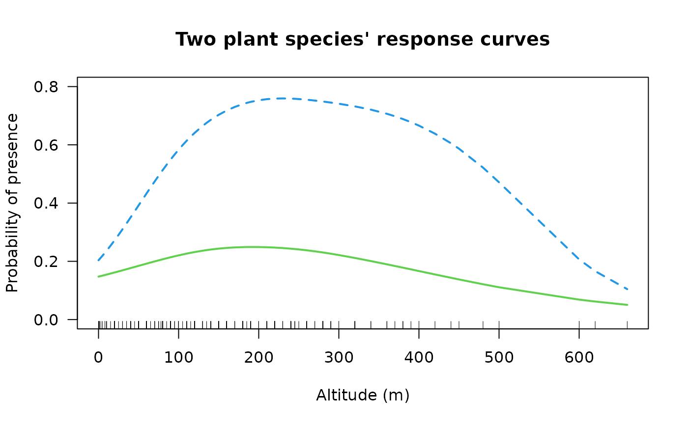
# Example 3; fit a two species GAM simultaneously
fit3 <- vgam(cbind(agaaus, kniexc) ~ s(altitude, df = c(2, 3)),
binomialff(multiple.responses = TRUE), data = hunua)
coef(fit3, matrix = TRUE) # Not really interpretable
#> logitlink(E[agaaus]) logitlink(E[kniexc])
#> (Intercept) -1.301849e+00 -0.072104658
#> s(altitude, df = c(2, 3)) 3.919179e-05 0.002721115
if (FALSE) plot(fit3, se = TRUE, overlay = TRUE, lcol = 3:4, scol = 3:4)
ooo <- with(hunua, order(altitude))
with(hunua, matplot(altitude[ooo], fitted(fit3)[ooo, ], type = "l",
lwd = 2, col = 3:4,
xlab = "Altitude (m)", ylab = "Probability of presence", las = 1,
main = "Two plant species' response curves", ylim = c(0, 0.8)))
with(hunua, rug(altitude)) # \dontrun{}
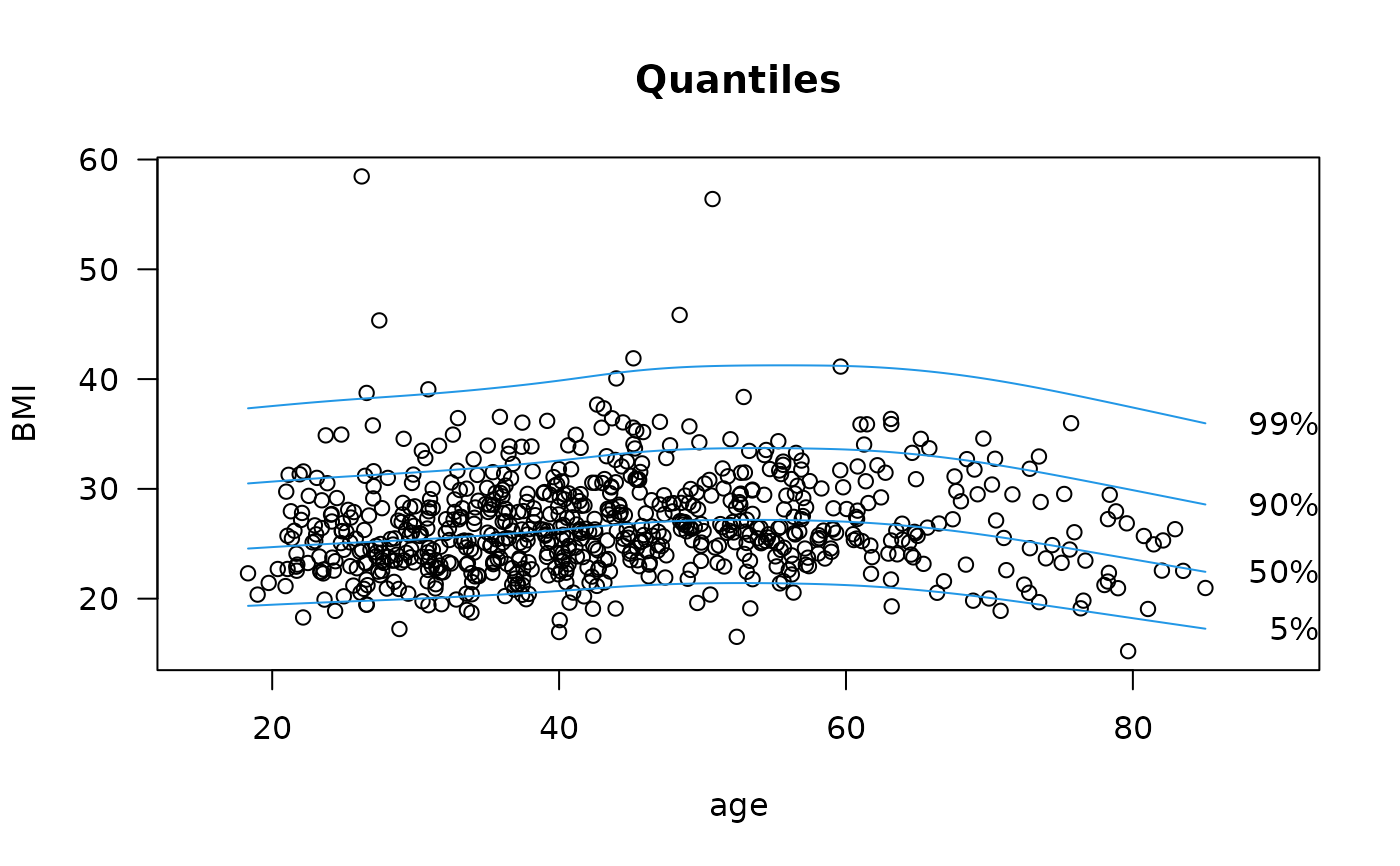
 # Example 4; LMS quantile regression
fit4 <- vgam(BMI ~ s(age, df = c(4, 2)), lms.bcn(zero = 1),
data = bmi.nz, trace = TRUE)
#> VGAM s.vam loop 1 : loglikelihood = -6429.7568
#> VGAM s.vam loop 2 : loglikelihood = -6327.3502
#> VGAM s.vam loop 3 : loglikelihood = -6313.2224
#> VGAM s.vam loop 4 : loglikelihood = -6312.8069
#> VGAM s.vam loop 5 : loglikelihood = -6312.8166
#> VGAM s.vam loop 6 : loglikelihood = -6312.8032
#> VGAM s.vam loop 7 : loglikelihood = -6312.8088
#> VGAM s.vam loop 8 : loglikelihood = -6312.8062
#> VGAM s.vam loop 9 : loglikelihood = -6312.8074
#> VGAM s.vam loop 10 : loglikelihood = -6312.8068
#> VGAM s.vam loop 11 : loglikelihood = -6312.8071
#> VGAM s.vam loop 12 : loglikelihood = -6312.807
head(predict(fit4))
#> lambda mu loglink(sigma)
#> 1 -0.6589584 25.48922 -1.851162
#> 2 -0.6589584 26.19783 -1.852918
#> 3 -0.6589584 26.66334 -1.853294
#> 4 -0.6589584 25.75937 -1.852382
#> 5 -0.6589584 27.17650 -1.852765
#> 6 -0.6589584 26.17517 -1.852911
head(fitted(fit4))
#> 25% 50% 75%
#> 1 23.00836 25.48922 28.44767
#> 2 23.65211 26.19783 29.23269
#> 3 24.07328 26.66334 29.75085
#> 4 23.25503 25.75937 28.74518
#> 5 24.53531 27.17650 30.32525
#> 6 23.63164 26.17517 29.20742
head(bmi.nz) # Person 1 is near the lower quartile among people his age
#> age BMI
#> 1 31.52966 22.77107
#> 2 39.38045 27.70033
#> 3 43.38940 28.18127
#> 4 34.84894 25.08380
#> 5 53.81990 26.46388
#> 6 39.17002 36.19648
head(cdf(fit4))
#> 1 2 3 4 5 6
#> 0.2280309 0.6365499 0.6356761 0.4321450 0.4321311 0.9686738
if (FALSE) par(mfrow = c(1,1), bty = "l", mar = c(5,4,4,3)+0.1, xpd=TRUE)
qtplot(fit4, percentiles = c(5,50,90,99), main = "Quantiles", las = 1,
xlim = c(15, 90), ylab = "BMI", lwd=2, lcol=4) # Quantile plot
# Example 4; LMS quantile regression
fit4 <- vgam(BMI ~ s(age, df = c(4, 2)), lms.bcn(zero = 1),
data = bmi.nz, trace = TRUE)
#> VGAM s.vam loop 1 : loglikelihood = -6429.7568
#> VGAM s.vam loop 2 : loglikelihood = -6327.3502
#> VGAM s.vam loop 3 : loglikelihood = -6313.2224
#> VGAM s.vam loop 4 : loglikelihood = -6312.8069
#> VGAM s.vam loop 5 : loglikelihood = -6312.8166
#> VGAM s.vam loop 6 : loglikelihood = -6312.8032
#> VGAM s.vam loop 7 : loglikelihood = -6312.8088
#> VGAM s.vam loop 8 : loglikelihood = -6312.8062
#> VGAM s.vam loop 9 : loglikelihood = -6312.8074
#> VGAM s.vam loop 10 : loglikelihood = -6312.8068
#> VGAM s.vam loop 11 : loglikelihood = -6312.8071
#> VGAM s.vam loop 12 : loglikelihood = -6312.807
head(predict(fit4))
#> lambda mu loglink(sigma)
#> 1 -0.6589584 25.48922 -1.851162
#> 2 -0.6589584 26.19783 -1.852918
#> 3 -0.6589584 26.66334 -1.853294
#> 4 -0.6589584 25.75937 -1.852382
#> 5 -0.6589584 27.17650 -1.852765
#> 6 -0.6589584 26.17517 -1.852911
head(fitted(fit4))
#> 25% 50% 75%
#> 1 23.00836 25.48922 28.44767
#> 2 23.65211 26.19783 29.23269
#> 3 24.07328 26.66334 29.75085
#> 4 23.25503 25.75937 28.74518
#> 5 24.53531 27.17650 30.32525
#> 6 23.63164 26.17517 29.20742
head(bmi.nz) # Person 1 is near the lower quartile among people his age
#> age BMI
#> 1 31.52966 22.77107
#> 2 39.38045 27.70033
#> 3 43.38940 28.18127
#> 4 34.84894 25.08380
#> 5 53.81990 26.46388
#> 6 39.17002 36.19648
head(cdf(fit4))
#> 1 2 3 4 5 6
#> 0.2280309 0.6365499 0.6356761 0.4321450 0.4321311 0.9686738
if (FALSE) par(mfrow = c(1,1), bty = "l", mar = c(5,4,4,3)+0.1, xpd=TRUE)
qtplot(fit4, percentiles = c(5,50,90,99), main = "Quantiles", las = 1,
xlim = c(15, 90), ylab = "BMI", lwd=2, lcol=4) # Quantile plot
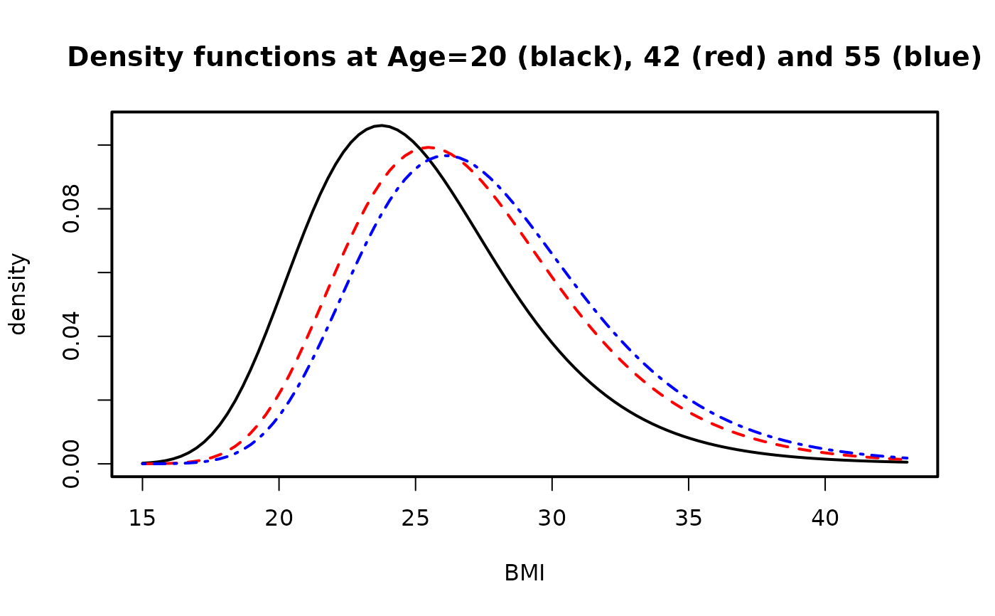
 ygrid <- seq(15, 43, len = 100) # BMI ranges
par(mfrow = c(1, 1), lwd = 2) # Density plot
aa <- deplot(fit4, x0 = 20, y = ygrid, xlab = "BMI", col = "black",
main = "Density functions at Age=20 (black), 42 (red) and 55 (blue)")
aa
#>
#> Call:
#> vgam(formula = BMI ~ s(age, df = c(4, 2)), family = lms.bcn(zero = 1),
#> data = bmi.nz, trace = TRUE)
#>
#>
#> Degrees of Freedom: 2100 Total; 2091.07 Residual
#> Log-likelihood: -6312.807
aa <- deplot(fit4, x0 = 42, y = ygrid, add = TRUE, llty = 2, col = "red")
aa <- deplot(fit4, x0 = 55, y = ygrid, add = TRUE, llty = 4, col = "blue",
Attach = TRUE)
ygrid <- seq(15, 43, len = 100) # BMI ranges
par(mfrow = c(1, 1), lwd = 2) # Density plot
aa <- deplot(fit4, x0 = 20, y = ygrid, xlab = "BMI", col = "black",
main = "Density functions at Age=20 (black), 42 (red) and 55 (blue)")
aa
#>
#> Call:
#> vgam(formula = BMI ~ s(age, df = c(4, 2)), family = lms.bcn(zero = 1),
#> data = bmi.nz, trace = TRUE)
#>
#>
#> Degrees of Freedom: 2100 Total; 2091.07 Residual
#> Log-likelihood: -6312.807
aa <- deplot(fit4, x0 = 42, y = ygrid, add = TRUE, llty = 2, col = "red")
aa <- deplot(fit4, x0 = 55, y = ygrid, add = TRUE, llty = 4, col = "blue",
Attach = TRUE)
 aa@post$deplot # Contains density function values
#> $newdata
#> age
#> 1 55
#>
#> $y
#> [1] 15.00000 15.28283 15.56566 15.84848 16.13131 16.41414 16.69697 16.97980
#> [9] 17.26263 17.54545 17.82828 18.11111 18.39394 18.67677 18.95960 19.24242
#> [17] 19.52525 19.80808 20.09091 20.37374 20.65657 20.93939 21.22222 21.50505
#> [25] 21.78788 22.07071 22.35354 22.63636 22.91919 23.20202 23.48485 23.76768
#> [33] 24.05051 24.33333 24.61616 24.89899 25.18182 25.46465 25.74747 26.03030
#> [41] 26.31313 26.59596 26.87879 27.16162 27.44444 27.72727 28.01010 28.29293
#> [49] 28.57576 28.85859 29.14141 29.42424 29.70707 29.98990 30.27273 30.55556
#> [57] 30.83838 31.12121 31.40404 31.68687 31.96970 32.25253 32.53535 32.81818
#> [65] 33.10101 33.38384 33.66667 33.94949 34.23232 34.51515 34.79798 35.08081
#> [73] 35.36364 35.64646 35.92929 36.21212 36.49495 36.77778 37.06061 37.34343
#> [81] 37.62626 37.90909 38.19192 38.47475 38.75758 39.04040 39.32323 39.60606
#> [89] 39.88889 40.17172 40.45455 40.73737 41.02020 41.30303 41.58586 41.86869
#> [97] 42.15152 42.43434 42.71717 43.00000
#>
#> $density
#> [1] 5.514476e-06 1.183736e-05 2.410571e-05 4.674236e-05 8.659734e-05
#> [6] 1.537653e-04 2.624337e-04 4.316555e-04 6.859150e-04 1.055349e-03
#> [11] 1.575500e-03 2.286505e-03 3.231706e-03 4.455686e-03 6.001866e-03
#> [16] 7.909800e-03 1.021239e-02 1.293322e-02 1.608430e-02 1.966432e-02
#> [21] 2.365757e-02 2.803374e-02 3.274839e-02 3.774427e-02 4.295318e-02
#> [26] 4.829847e-02 5.369773e-02 5.906576e-02 6.431749e-02 6.937072e-02
#> [31] 7.414863e-02 7.858188e-02 8.261025e-02 8.618386e-02 8.926386e-02
#> [36] 9.182275e-02 9.384416e-02 9.532247e-02 9.626195e-02 9.667582e-02
#> [41] 9.658509e-02 9.601735e-02 9.500546e-02 9.358636e-02 9.179984e-02
#> [46] 8.968741e-02 8.729134e-02 8.465373e-02 8.181578e-02 7.881714e-02
#> [51] 7.569540e-02 7.248573e-02 6.922057e-02 6.592948e-02 6.263902e-02
#> [56] 5.937275e-02 5.615129e-02 5.299237e-02 4.991098e-02 4.691958e-02
#> [61] 4.402819e-02 4.124469e-02 3.857493e-02 3.602300e-02 3.359141e-02
#> [66] 3.128127e-02 2.909250e-02 2.702397e-02 2.507369e-02 2.323897e-02
#> [71] 2.151651e-02 1.990255e-02 1.839299e-02 1.698346e-02 1.566939e-02
#> [76] 1.444614e-02 1.330901e-02 1.225331e-02 1.127439e-02 1.036770e-02
#> [81] 9.528813e-03 8.753430e-03 8.037412e-03 7.376792e-03 6.767782e-03
#> [86] 6.206777e-03 5.690362e-03 5.215306e-03 4.778569e-03 4.377289e-03
#> [91] 4.008785e-03 3.670547e-03 3.360231e-03 3.075652e-03 2.814777e-03
#> [96] 2.575718e-03 2.356722e-03 2.156164e-03 1.972543e-03 1.804468e-03
#>
# \dontrun{}
# Example 5; GEV distribution for extremes
(fit5 <- vglm(maxtemp ~ 1, gevff, data = oxtemp, trace = TRUE))
#> Iteration 1: loglikelihood = -228.90576
#> Iteration 2: loglikelihood = -228.89653
#> Iteration 3: loglikelihood = -228.89652
#> Iteration 4: loglikelihood = -228.89652
#>
#> Call:
#> vglm(formula = maxtemp ~ 1, family = gevff, data = oxtemp, trace = TRUE)
#>
#>
#> Coefficients:
#> (Intercept):1 (Intercept):2 (Intercept):3
#> 83.838467 1.449270 -1.547556
#>
#> Degrees of Freedom: 240 Total; 237 Residual
#> Log-likelihood: -228.8965
head(fitted(fit5))
#> 95% 99%
#> 1 92.35044 94.71293
#> 2 92.35044 94.71293
#> 3 92.35044 94.71293
#> 4 92.35044 94.71293
#> 5 92.35044 94.71293
#> 6 92.35044 94.71293
coef(fit5, matrix = TRUE)
#> location loglink(scale) logofflink(shape, offset = 0.5)
#> (Intercept) 83.83847 1.44927 -1.547556
Coef(fit5)
#> location scale shape
#> 83.8384672 4.2600036 -0.2872327
vcov(fit5)
#> (Intercept):1 (Intercept):2 (Intercept):3
#> (Intercept):1 0.2669002973 -0.0009746616 -0.04928180
#> (Intercept):2 -0.0009746616 0.0072373297 -0.01358841
#> (Intercept):3 -0.0492818027 -0.0135884143 0.07543028
vcov(fit5, untransform = TRUE)
#> location scale shape
#> location 0.266900297 -0.004152062 -0.010485558
#> scale -0.004152062 0.131340385 -0.012316398
#> shape -0.010485558 -0.012316398 0.003414724
sqrt(diag(vcov(fit5))) # Approximate standard errors
#> (Intercept):1 (Intercept):2 (Intercept):3
#> 0.5166239 0.0850725 0.2746457
if (FALSE) rlplot(fit5) # \dontrun{}
aa@post$deplot # Contains density function values
#> $newdata
#> age
#> 1 55
#>
#> $y
#> [1] 15.00000 15.28283 15.56566 15.84848 16.13131 16.41414 16.69697 16.97980
#> [9] 17.26263 17.54545 17.82828 18.11111 18.39394 18.67677 18.95960 19.24242
#> [17] 19.52525 19.80808 20.09091 20.37374 20.65657 20.93939 21.22222 21.50505
#> [25] 21.78788 22.07071 22.35354 22.63636 22.91919 23.20202 23.48485 23.76768
#> [33] 24.05051 24.33333 24.61616 24.89899 25.18182 25.46465 25.74747 26.03030
#> [41] 26.31313 26.59596 26.87879 27.16162 27.44444 27.72727 28.01010 28.29293
#> [49] 28.57576 28.85859 29.14141 29.42424 29.70707 29.98990 30.27273 30.55556
#> [57] 30.83838 31.12121 31.40404 31.68687 31.96970 32.25253 32.53535 32.81818
#> [65] 33.10101 33.38384 33.66667 33.94949 34.23232 34.51515 34.79798 35.08081
#> [73] 35.36364 35.64646 35.92929 36.21212 36.49495 36.77778 37.06061 37.34343
#> [81] 37.62626 37.90909 38.19192 38.47475 38.75758 39.04040 39.32323 39.60606
#> [89] 39.88889 40.17172 40.45455 40.73737 41.02020 41.30303 41.58586 41.86869
#> [97] 42.15152 42.43434 42.71717 43.00000
#>
#> $density
#> [1] 5.514476e-06 1.183736e-05 2.410571e-05 4.674236e-05 8.659734e-05
#> [6] 1.537653e-04 2.624337e-04 4.316555e-04 6.859150e-04 1.055349e-03
#> [11] 1.575500e-03 2.286505e-03 3.231706e-03 4.455686e-03 6.001866e-03
#> [16] 7.909800e-03 1.021239e-02 1.293322e-02 1.608430e-02 1.966432e-02
#> [21] 2.365757e-02 2.803374e-02 3.274839e-02 3.774427e-02 4.295318e-02
#> [26] 4.829847e-02 5.369773e-02 5.906576e-02 6.431749e-02 6.937072e-02
#> [31] 7.414863e-02 7.858188e-02 8.261025e-02 8.618386e-02 8.926386e-02
#> [36] 9.182275e-02 9.384416e-02 9.532247e-02 9.626195e-02 9.667582e-02
#> [41] 9.658509e-02 9.601735e-02 9.500546e-02 9.358636e-02 9.179984e-02
#> [46] 8.968741e-02 8.729134e-02 8.465373e-02 8.181578e-02 7.881714e-02
#> [51] 7.569540e-02 7.248573e-02 6.922057e-02 6.592948e-02 6.263902e-02
#> [56] 5.937275e-02 5.615129e-02 5.299237e-02 4.991098e-02 4.691958e-02
#> [61] 4.402819e-02 4.124469e-02 3.857493e-02 3.602300e-02 3.359141e-02
#> [66] 3.128127e-02 2.909250e-02 2.702397e-02 2.507369e-02 2.323897e-02
#> [71] 2.151651e-02 1.990255e-02 1.839299e-02 1.698346e-02 1.566939e-02
#> [76] 1.444614e-02 1.330901e-02 1.225331e-02 1.127439e-02 1.036770e-02
#> [81] 9.528813e-03 8.753430e-03 8.037412e-03 7.376792e-03 6.767782e-03
#> [86] 6.206777e-03 5.690362e-03 5.215306e-03 4.778569e-03 4.377289e-03
#> [91] 4.008785e-03 3.670547e-03 3.360231e-03 3.075652e-03 2.814777e-03
#> [96] 2.575718e-03 2.356722e-03 2.156164e-03 1.972543e-03 1.804468e-03
#>
# \dontrun{}
# Example 5; GEV distribution for extremes
(fit5 <- vglm(maxtemp ~ 1, gevff, data = oxtemp, trace = TRUE))
#> Iteration 1: loglikelihood = -228.90576
#> Iteration 2: loglikelihood = -228.89653
#> Iteration 3: loglikelihood = -228.89652
#> Iteration 4: loglikelihood = -228.89652
#>
#> Call:
#> vglm(formula = maxtemp ~ 1, family = gevff, data = oxtemp, trace = TRUE)
#>
#>
#> Coefficients:
#> (Intercept):1 (Intercept):2 (Intercept):3
#> 83.838467 1.449270 -1.547556
#>
#> Degrees of Freedom: 240 Total; 237 Residual
#> Log-likelihood: -228.8965
head(fitted(fit5))
#> 95% 99%
#> 1 92.35044 94.71293
#> 2 92.35044 94.71293
#> 3 92.35044 94.71293
#> 4 92.35044 94.71293
#> 5 92.35044 94.71293
#> 6 92.35044 94.71293
coef(fit5, matrix = TRUE)
#> location loglink(scale) logofflink(shape, offset = 0.5)
#> (Intercept) 83.83847 1.44927 -1.547556
Coef(fit5)
#> location scale shape
#> 83.8384672 4.2600036 -0.2872327
vcov(fit5)
#> (Intercept):1 (Intercept):2 (Intercept):3
#> (Intercept):1 0.2669002973 -0.0009746616 -0.04928180
#> (Intercept):2 -0.0009746616 0.0072373297 -0.01358841
#> (Intercept):3 -0.0492818027 -0.0135884143 0.07543028
vcov(fit5, untransform = TRUE)
#> location scale shape
#> location 0.266900297 -0.004152062 -0.010485558
#> scale -0.004152062 0.131340385 -0.012316398
#> shape -0.010485558 -0.012316398 0.003414724
sqrt(diag(vcov(fit5))) # Approximate standard errors
#> (Intercept):1 (Intercept):2 (Intercept):3
#> 0.5166239 0.0850725 0.2746457
if (FALSE) rlplot(fit5) # \dontrun{}