Censored Gumbel Distribution

Maximum likelihood estimation of the 2-parameter Gumbel distribution when there are censored observations. A matrix response is not allowed.

cens.gumbel(llocation = "identitylink", lscale = "loglink",
            iscale = NULL, mean = TRUE, percentiles = NULL,
            zero = "scale")

Arguments

llocation, lscale

Character. Parameter link functions for the location and (positive) \(scale\) parameters. See Links for more choices.

iscale

Numeric and positive. Initial value for \(scale\). Recycled to the appropriate length. In general, a larger value is better than a smaller value. The default is to choose the value internally.

mean

Logical. Return the mean? If TRUE then the mean is returned, otherwise percentiles given by the percentiles argument.

percentiles

Numeric with values between 0 and 100. If mean=FALSE then the fitted values are percentiles which must be specified by this argument.

zero

An integer-valued vector specifying which linear/additive predictors are modelled as intercepts only. The value (possibly values) must be from the set {1,2} corresponding respectively to \(location\) and \(scale\). If zero=NULL then all linear/additive predictors are modelled as a linear combination of the explanatory variables. The default is to fit the shape parameter as an intercept only. See CommonVGAMffArguments for more information.

Details

This VGAM family function is like gumbel but handles observations that are left-censored (so that the true value would be less than the observed value) else right-censored (so that the true value would be greater than the observed value). To indicate which type of censoring, input extra = list(leftcensored = vec1, rightcensored = vec2) where vec1 and vec2 are logical vectors the same length as the response. If the two components of this list are missing then the logical values are taken to be FALSE. The fitted object has these two components stored in the extra slot.

Value

An object of class "vglmff" (see vglmff-class). The object is used by modelling functions such as vglm and vgam.

References

Coles, S. (2001). An Introduction to Statistical Modeling of Extreme Values. London: Springer-Verlag.

Author

T. W. Yee

Warning

Numerical problems may occur if the amount of censoring is excessive.

Note

See gumbel for details about the Gumbel distribution. The initial values are based on assuming all uncensored observations, therefore could be improved upon.

See also

gumbel, gumbelff, rgumbel, guplot, gev, venice.

Examples

# Example 1
ystar <- venice[["r1"]]  # Use the first order statistic as the response
nn <- length(ystar)
L <- runif(nn, 100, 104)  # Lower censoring points
U <- runif(nn, 130, 135)  # Upper censoring points
y <- pmax(L, ystar)  # Left  censored
y <- pmin(U, y)      # Right censored
extra <- list(leftcensored = ystar < L, rightcensored = ystar > U)
fit <- vglm(y ~ scale(year), data = venice, trace = TRUE, extra = extra,
            fam = cens.gumbel(mean = FALSE, perc = c(5, 25, 50, 75, 95)))
#> Iteration 1: loglikelihood = -160.97954
#> Iteration 2: loglikelihood = -148.06843
#> Iteration 3: loglikelihood = -147.41345
#> Iteration 4: loglikelihood = -147.3925
#> Iteration 5: loglikelihood = -147.38886
#> Iteration 6: loglikelihood = -147.38795
#> Iteration 7: loglikelihood = -147.38772
#> Iteration 8: loglikelihood = -147.38766
#> Iteration 9: loglikelihood = -147.38765
#> Iteration 10: loglikelihood = -147.38765
#> Iteration 11: loglikelihood = -147.38765
coef(fit, matrix = TRUE)
#>               location loglink(scale)
#> (Intercept) 112.534500       2.617486
#> scale(year)   7.666845       0.000000
head(fitted(fit))
#>         5%      25%      50%      75%      95%
#> 1 84.60846 95.16601 104.6630 116.7117 140.3367
#> 2 85.12419 95.68174 105.1787 117.2274 140.8524
#> 3 85.63992 96.19747 105.6944 117.7431 141.3681
#> 4 86.15565 96.71320 106.2102 118.2588 141.8838
#> 5 86.67137 97.22892 106.7259 118.7746 142.3996
#> 6 87.18710 97.74465 107.2416 119.2903 142.9153
fit@extra
#> $leftcensored
#>  [1] FALSE  TRUE FALSE FALSE FALSE FALSE FALSE FALSE  TRUE FALSE  TRUE  TRUE
#> [13]  TRUE FALSE FALSE FALSE FALSE FALSE FALSE FALSE FALSE FALSE FALSE FALSE
#> [25]  TRUE  TRUE FALSE FALSE FALSE FALSE FALSE FALSE FALSE FALSE FALSE FALSE
#> [37] FALSE FALSE FALSE FALSE FALSE FALSE FALSE  TRUE FALSE FALSE FALSE FALSE
#> [49] FALSE FALSE FALSE
#> 
#> $rightcensored
#>  [1] FALSE FALSE FALSE FALSE FALSE  TRUE FALSE FALSE FALSE FALSE FALSE FALSE
#> [13] FALSE FALSE FALSE  TRUE FALSE FALSE FALSE FALSE  TRUE FALSE FALSE FALSE
#> [25] FALSE FALSE FALSE FALSE FALSE  TRUE FALSE FALSE FALSE FALSE FALSE  TRUE
#> [37]  TRUE  TRUE  TRUE FALSE FALSE FALSE FALSE FALSE FALSE FALSE FALSE  TRUE
#> [49]  TRUE  TRUE  TRUE
#> 

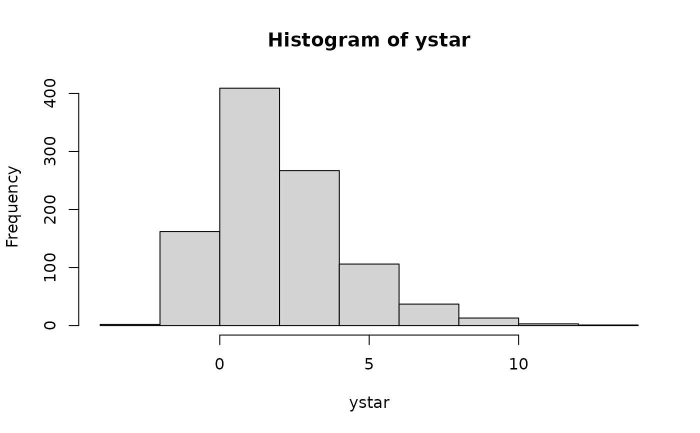
# Example 2: simulated data
nn <- 1000
ystar <- rgumbel(nn, loc = 1, scale = exp(0.5))  # The uncensored data
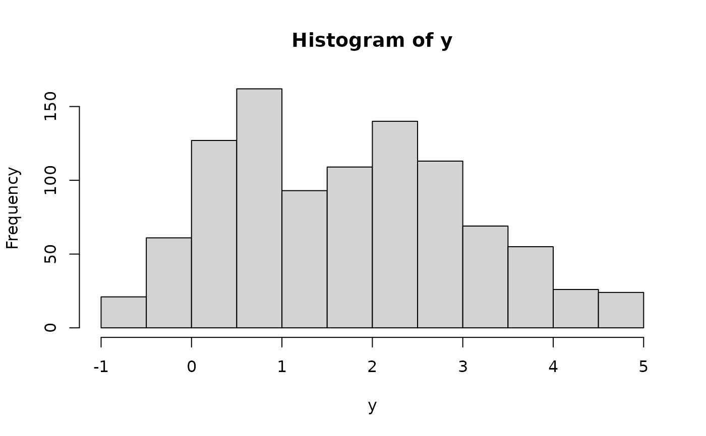
L <- runif(nn, -1, 1)  # Lower censoring points
U <- runif(nn,  2, 5)  # Upper censoring points
y <- pmax(L, ystar)  # Left  censored
y <- pmin(U, y)      # Right censored
if (FALSE) par(mfrow = c(1, 2)); hist(ystar); hist(y); # \dontrun{}


extra <- list(leftcensored = ystar < L, rightcensored = ystar > U)
fit <- vglm(y ~ 1, trace = TRUE, extra = extra, fam = cens.gumbel)
#> Iteration 1: loglikelihood = -1961.5616
#> Iteration 2: loglikelihood = -1640.4276
#> Iteration 3: loglikelihood = -1635.915
#> Iteration 4: loglikelihood = -1634.9063
#> Iteration 5: loglikelihood = -1634.664
#> Iteration 6: loglikelihood = -1634.6097
#> Iteration 7: loglikelihood = -1634.5981
#> Iteration 8: loglikelihood = -1634.5956
#> Iteration 9: loglikelihood = -1634.5951
#> Iteration 10: loglikelihood = -1634.595
#> Iteration 11: loglikelihood = -1634.5949
#> Iteration 12: loglikelihood = -1634.5949
coef(fit, matrix = TRUE)
#>             location loglink(scale)
#> (Intercept) 1.014301      0.5136358