Confidence of Mock Jurors in Their Verdicts

Data with responses of naive mock jurors to the conventional conventional two-option verdict (guilt vs. acquittal) versus a three-option verdict setup (the third option was the Scottish 'not proven' alternative), in the presence/absence of conflicting testimonial evidence.

Usage

data("MockJurors", package = "betareg")

Format

A data frame containing 104 observations on 3 variables.

verdict: factor indicating whether a two-option or three-option verdict is requested. (A sum contrast rather than treatment contrast is employed.)
conflict: factor. Is there conflicting testimonial evidence? (A sum contrast rather than treatment contrast is employed.)
confidence: jurors degree of confidence in his/her verdict, scaled to the open unit interval (see below).

Details

The data were collected by Daily (2004) among first-year psychology students at Australian National University. Smithson and Verkuilen (2006) employed the data scaling the original confidence (on a scale 0–100) to the open unit interval: ((original_confidence/100) * 103 - 0.5) / 104.

The original coding of conflict in the data provided from Smithson's homepage is -1/1 which Smithson and Verkuilen (2006) describe to mean no/yes. However, all their results (sample statistics, histograms, etc.) suggest that it actually means yes/no which was employed in MockJurors.

Source

Example 1 from Smithson and Verkuilen (2006) supplements.

References

Deady S (2004). The Psychological Third Verdict: 'Not Proven' or 'Not Willing to Make a Decision'? Unpublished honors thesis, The Australian National University, Canberra.

Smithson M, Verkuilen J (2006). A Better Lemon Squeezer? Maximum-Likelihood Regression with Beta-Distributed Dependent Variables. Psychological Methods, 11(7), 54–71.

Examples

data("MockJurors", package = "betareg")
library("lmtest")

## Smithson & Verkuilen (2006, Table 1)
## variable dispersion model
## (NOTE: numerical rather than analytical Hessian is used for replication,
##  Smithson & Verkuilen erroneously compute one-sided p-values)
mj_vd <- betareg(confidence ~ verdict * conflict | verdict * conflict,
  data = MockJurors, hessian = TRUE)
summary(mj_vd)
#> 
#> Call:
#> betareg(formula = confidence ~ verdict * conflict | verdict * conflict, 
#>     data = MockJurors, hessian = TRUE)
#> 
#> Quantile residuals:
#>    Min     1Q Median     3Q    Max 
#> -2.476 -0.665 -0.099  0.600  2.644 
#> 
#> Coefficients (mean model with logit link):
#>                  Estimate Std. Error z value Pr(>|z|)    
#> (Intercept)       0.91240    0.10398    8.77   <2e-16 ***
#> verdict           0.00504    0.10398    0.05   0.9614    
#> conflict          0.16857    0.10398    1.62   0.1050    
#> verdict:conflict  0.28001    0.10398    2.69   0.0071 ** 
#> 
#> Phi coefficients (precision model with log link):
#>                  Estimate Std. Error z value Pr(>|z|)    
#> (Intercept)         1.173      0.128    9.18   <2e-16 ***
#> verdict            -0.330      0.128   -2.58   0.0099 ** 
#> conflict            0.220      0.128    1.72   0.0858 .  
#> verdict:conflict    0.316      0.128    2.47   0.0133 *  
#> ---
#> Signif. codes:  0 '***' 0.001 '**' 0.01 '*' 0.05 '.' 0.1 ' ' 1 
#> 
#> Type of estimator: ML (maximum likelihood)
#> Log-likelihood: 40.1 on 8 Df
#> Pseudo R-squared: 0.0389
#> Number of iterations in BFGS optimization: 19 

## model selection for beta regression: null model, fixed dispersion model (p. 61)
mj_null <- betareg(confidence ~ 1 | 1, data = MockJurors)
mj_fd <-   betareg(confidence ~ verdict * conflict | 1, data = MockJurors)
lrtest(mj_null, mj_fd)
#> Likelihood ratio test
#> 
#> Model 1: confidence ~ 1 | 1
#> Model 2: confidence ~ verdict * conflict | 1
#>   #Df LogLik Df Chisq Pr(>Chisq)
#> 1   2   28.2                    
#> 2   5   30.6  3  4.71       0.19
lrtest(mj_null, mj_vd)
#> Likelihood ratio test
#> 
#> Model 1: confidence ~ 1 | 1
#> Model 2: confidence ~ verdict * conflict | verdict * conflict
#>   #Df LogLik Df Chisq Pr(>Chisq)    
#> 1   2   28.2                        
#> 2   8   40.1  6  23.8    0.00057 ***
#> ---
#> Signif. codes:  0 ‘***’ 0.001 ‘**’ 0.01 ‘*’ 0.05 ‘.’ 0.1 ‘ ’ 1
## McFadden's pseudo-R-squared
1 - as.vector(logLik(mj_null)/logLik(mj_vd))
#> [1] 0.2964

## visualization
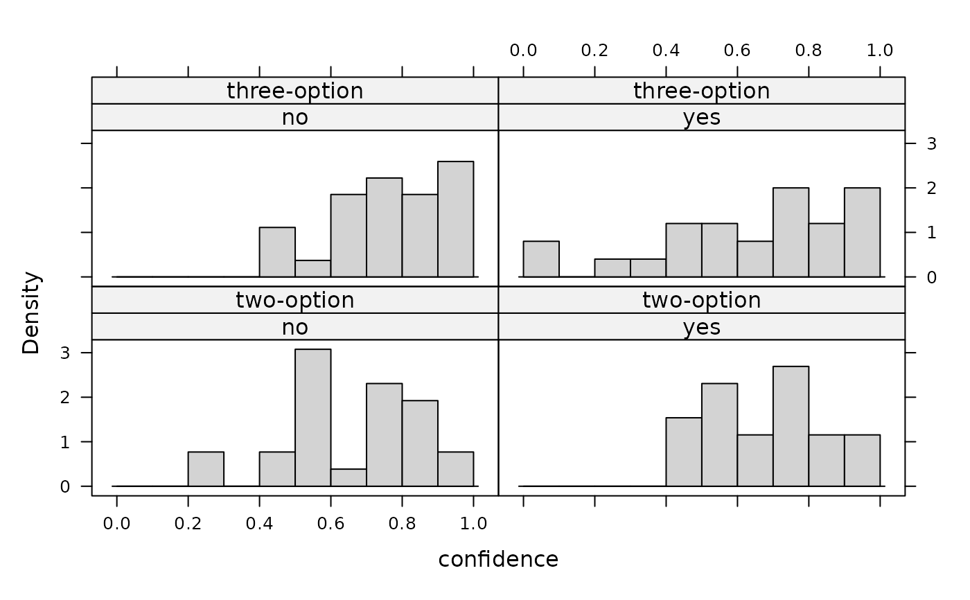
if(require("lattice")) {
  histogram(~ confidence | conflict + verdict, data = MockJurors,
    col = "lightgray", breaks = 0:10/10, type = "density")
}
#> Loading required package: lattice


## see demo("SmithsonVerkuilen2006", package = "betareg") for more details