Dependency of Anxiety on Stress

Stress and anxiety among nonclinical women in Townsville, Queensland, Australia.

Usage

data("StressAnxiety", package = "betareg")

Format

A data frame containing 166 observations on 2 variables.

stress: score, linearly transformed to the open unit interval (see below).
anxiety: score, linearly transformed to the open unit interval (see below).

Details

Both variables were assess on the Depression Anxiety Stress Scales, ranging from 0 to 42. Smithson and Verkuilen (2006) transformed these to the open unit interval (without providing details about this transformation).

Source

Example 2 from Smithson and Verkuilen (2006) supplements.

References

Smithson M, Verkuilen J (2006). A Better Lemon Squeezer? Maximum-Likelihood Regression with Beta-Distributed Dependent Variables. Psychological Methods, 11(7), 54–71.

Examples

data("StressAnxiety", package = "betareg")
StressAnxiety <- StressAnxiety[order(StressAnxiety$stress),]

## Smithson & Verkuilen (2006, Table 4)
sa_null <- betareg(anxiety ~ 1 | 1,
  data = StressAnxiety, hessian = TRUE)
sa_stress <- betareg(anxiety ~ stress | stress,
  data = StressAnxiety, hessian = TRUE)
summary(sa_null)
#> 
#> Call:
#> betareg(formula = anxiety ~ 1 | 1, data = StressAnxiety, hessian = TRUE)
#> 
#> Quantile residuals:
#>    Min     1Q Median     3Q    Max 
#> -0.838 -0.838 -0.447  0.622  3.240 
#> 
#> Coefficients (mean model with logit link):
#>             Estimate Std. Error z value Pr(>|z|)    
#> (Intercept)  -2.2440     0.0988   -22.7   <2e-16 ***
#> 
#> Phi coefficients (precision model with log link):
#>             Estimate Std. Error z value Pr(>|z|)    
#> (Intercept)    1.796      0.123    14.6   <2e-16 ***
#> ---
#> Signif. codes:  0 '***' 0.001 '**' 0.01 '*' 0.05 '.' 0.1 ' ' 1 
#> 
#> Type of estimator: ML (maximum likelihood)
#> Log-likelihood:  239 on 2 Df
#> Number of iterations in BFGS optimization: 9 
summary(sa_stress)
#> 
#> Call:
#> betareg(formula = anxiety ~ stress | stress, data = StressAnxiety, hessian = TRUE)
#> 
#> Quantile residuals:
#>    Min     1Q Median     3Q    Max 
#> -2.012 -0.795 -0.183  0.566  3.114 
#> 
#> Coefficients (mean model with logit link):
#>             Estimate Std. Error z value Pr(>|z|)    
#> (Intercept)   -4.024      0.144   -27.9   <2e-16 ***
#> stress         4.941      0.441    11.2   <2e-16 ***
#> 
#> Phi coefficients (precision model with log link):
#>             Estimate Std. Error z value Pr(>|z|)    
#> (Intercept)    3.961      0.251   15.78  < 2e-16 ***
#> stress        -4.273      0.753   -5.67  1.4e-08 ***
#> ---
#> Signif. codes:  0 '***' 0.001 '**' 0.01 '*' 0.05 '.' 0.1 ' ' 1 
#> 
#> Type of estimator: ML (maximum likelihood)
#> Log-likelihood:  302 on 4 Df
#> Pseudo R-squared: 0.475
#> Number of iterations in BFGS optimization: 16 
AIC(sa_null, sa_stress)
#>           df    AIC
#> sa_null    2 -474.9
#> sa_stress  4 -595.9
1 - as.vector(logLik(sa_null)/logLik(sa_stress))
#> [1] 0.207

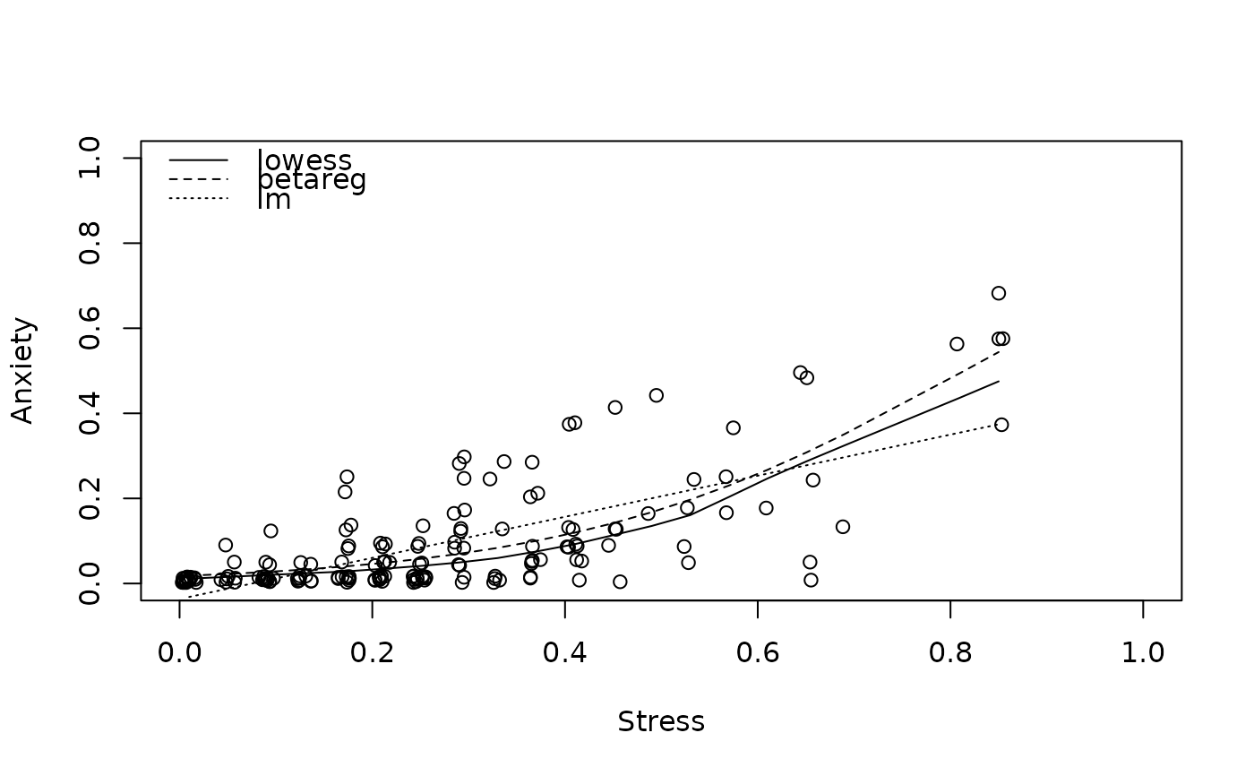
## visualization
attach(StressAnxiety)
plot(jitter(anxiety) ~ jitter(stress),
  xlab = "Stress", ylab = "Anxiety",
  xlim = c(0, 1), ylim = c(0, 1))
lines(lowess(anxiety ~ stress))
lines(fitted(sa_stress) ~ stress, lty = 2)
lines(fitted(lm(anxiety ~ stress)) ~ stress, lty = 3)
legend("topleft", c("lowess", "betareg", "lm"), lty = 1:3, bty = "n")

detach(StressAnxiety)

## see demo("SmithsonVerkuilen2006", package = "betareg") for more details