Dyslexia and IQ Predicting Reading Accuracy
ReadingSkills.RdData for assessing the contribution of non-verbal IQ to children's reading skills in dyslexic and non-dyslexic children.
Usage
data("ReadingSkills", package = "betareg")Format
A data frame containing 44 observations on 3 variables.
- accuracy
numeric. Reading score with maximum restricted to be 0.99 rather than 1 (see below).
- dyslexia
factor. Is the child dyslexic? (A sum contrast rather than treatment contrast is employed.)
- iq
numeric. Non-verbal intelligence quotient transformed to z-scores.
- accuracy1
numeric. Unrestricted reading score with a maximum of 1 (see below).
Details
The data were collected by Pammer and Kevan (2004) and employed by
Smithson and Verkuilen (2006). The original reading accuracy score was transformed
by Smithson and Verkuilen (2006) so that accuracy is in the open unit
interval (0, 1) and beta regression can be employed. First, the original accuracy
was scaled using the minimal and maximal score (a and b, respectively)
that can be obtained in the test: accuracy1 = (original_accuracy - a) / (b - a)
(a and b are not provided). Subsequently, accuracy was obtained
from accuracy1 by replacing all observations with a value of 1 with 0.99.
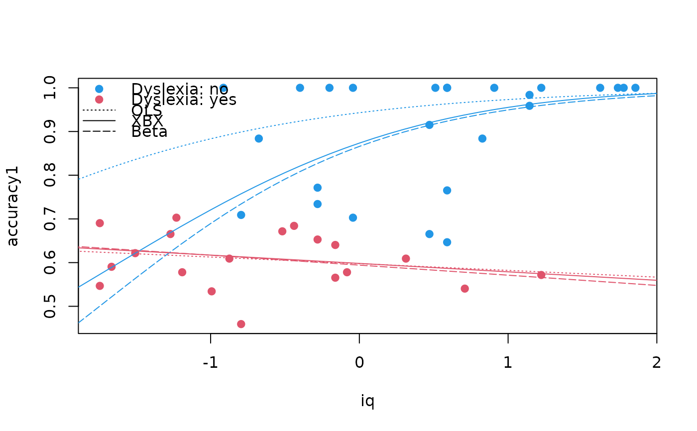
Kosmidis and Zeileis (2026) propose to investigate the original unrestricted
accuracy1 variable using their extended-support beta mixture regression.
References
Cribari-Neto F, Zeileis A (2010). Beta Regression in R. Journal of Statistical Software, 34(2), 1–24. doi:10.18637/jss.v034.i02
Grün B, Kosmidis I, Zeileis A (2012). Extended Beta Regression in R: Shaken, Stirred, Mixed, and Partitioned. Journal of Statistical Software, 48(11), 1–25. doi:10.18637/jss.v048.i11
Kosmidis I, Zeileis A (2026). Extended-Support Beta Regression for [0, 1] Responses. Journal of the Royal Statistical Society C, 75(1), 139–157. doi:10.1093/jrsssc/qlaf039
Pammer K, Kevan A (2004). The Contribution of Visual Sensitivity, Phonological Processing and Non-Verbal IQ to Children's Reading. Unpublished manuscript, The Australian National University, Canberra.
Smithson M, Verkuilen J (2006). A Better Lemon Squeezer? Maximum-Likelihood Regression with Beta-Distributed Dependent Variables. Psychological Methods, 11(7), 54–71.
Examples
options(digits = 4)
data("ReadingSkills", package = "betareg")
## Smithson & Verkuilen (2006, Table 5)
## OLS regression
## (Note: typo in iq coefficient: 0.3954 instead of 0.3594)
rs_ols <- lm(qlogis(accuracy) ~ dyslexia * iq, data = ReadingSkills)
summary(rs_ols)
#>
#> Call:
#> lm(formula = qlogis(accuracy) ~ dyslexia * iq, data = ReadingSkills)
#>
#> Residuals:
#> Min 1Q Median 3Q Max
#> -2.6640 -0.3797 0.0369 0.4089 2.5035
#>
#> Coefficients:
#> Estimate Std. Error t value Pr(>|t|)
#> (Intercept) 1.601 0.226 7.09 1.4e-08 ***
#> dyslexia -1.206 0.226 -5.34 4.0e-06 ***
#> iq 0.359 0.225 1.59 0.119
#> dyslexia:iq -0.423 0.225 -1.88 0.068 .
#> ---
#> Signif. codes: 0 ‘***’ 0.001 ‘**’ 0.01 ‘*’ 0.05 ‘.’ 0.1 ‘ ’ 1
#>
#> Residual standard error: 1.2 on 40 degrees of freedom
#> Multiple R-squared: 0.615, Adjusted R-squared: 0.586
#> F-statistic: 21.3 on 3 and 40 DF, p-value: 2.08e-08
#>
## Beta regression (with numerical rather than analytic standard errors)
## (Note: Smithson & Verkuilen erroneously compute one-sided p-values)
rs_beta <- betareg(accuracy ~ dyslexia * iq | dyslexia + iq,
data = ReadingSkills, hessian = TRUE)
summary(rs_beta)
#>
#> Call:
#> betareg(formula = accuracy ~ dyslexia * iq | dyslexia + iq, data = ReadingSkills,
#> hessian = TRUE)
#>
#> Quantile residuals:
#> Min 1Q Median 3Q Max
#> -2.362 -0.587 0.303 0.942 1.587
#>
#> Coefficients (mean model with logit link):
#> Estimate Std. Error z value Pr(>|z|)
#> (Intercept) 1.123 0.151 7.44 9.8e-14 ***
#> dyslexia -0.742 0.151 -4.90 9.7e-07 ***
#> iq 0.486 0.167 2.91 0.00360 **
#> dyslexia:iq -0.581 0.173 -3.37 0.00076 ***
#>
#> Phi coefficients (precision model with log link):
#> Estimate Std. Error z value Pr(>|z|)
#> (Intercept) 3.304 0.227 14.59 < 2e-16 ***
#> dyslexia 1.747 0.294 5.94 2.8e-09 ***
#> iq 1.229 0.460 2.67 0.0075 **
#> ---
#> Signif. codes: 0 '***' 0.001 '**' 0.01 '*' 0.05 '.' 0.1 ' ' 1
#>
#> Type of estimator: ML (maximum likelihood)
#> Log-likelihood: 65.9 on 7 Df
#> Pseudo R-squared: 0.576
#> Number of iterations in BFGS optimization: 25
## Extended-support beta mixture regression (Kosmidis & Zeileis 2026)
rs_xbx <- betareg(accuracy1 ~ dyslexia * iq | dyslexia + iq, data = ReadingSkills)
summary(rs_xbx)
#>
#> Call:
#> betareg(formula = accuracy1 ~ dyslexia * iq | dyslexia + iq, data = ReadingSkills)
#>
#> Randomized quantile residuals:
#> Min 1Q Median 3Q Max
#> -2.418 -0.598 -0.007 0.713 1.272
#>
#> Coefficients (mu model with logit link):
#> Estimate Std. Error z value Pr(>|z|)
#> (Intercept) 0.903 0.217 4.17 3.1e-05 ***
#> dyslexia -0.606 0.182 -3.34 0.00084 ***
#> iq 0.329 0.188 1.75 0.07989 .
#> dyslexia:iq -0.388 0.199 -1.94 0.05205 .
#>
#> Phi coefficients (phi model with log link):
#> Estimate Std. Error z value Pr(>|z|)
#> (Intercept) 3.499 0.530 6.60 4.1e-11 ***
#> dyslexia 1.736 0.449 3.86 0.00011 ***
#> iq 0.697 0.571 1.22 0.22243
#>
#> Exceedence parameter (extended-support xbetax model):
#> Estimate Std. Error z value Pr(>|z|)
#> Log(nu) -1.790 0.854 -2.1 0.036 *
#> ---
#> Signif. codes: 0 '***' 0.001 '**' 0.01 '*' 0.05 '.' 0.1 ' ' 1
#>
#> Exceedence parameter nu: 0.167
#> Type of estimator: ML (maximum likelihood)
#> Log-likelihood: 18.5 on 8 Df
#> Number of iterations in BFGS optimization: 29
## Coefficients in XBX are typically somewhat shrunken compared to beta
cbind(XBX = coef(rs_xbx), Beta = c(coef(rs_beta), NA))
#> XBX Beta
#> (Intercept) 0.9030 1.1232
#> dyslexia -0.6065 -0.7416
#> iq 0.3288 0.4864
#> dyslexia:iq -0.3875 -0.5813
#> (phi)_(Intercept) 3.4990 3.3044
#> (phi)_dyslexia 1.7360 1.7466
#> (phi)_iq 0.6965 1.2291
#> Log(nu) -1.7905 NA
## Visualization
plot(accuracy1 ~ iq, data = ReadingSkills, col = c(4, 2)[dyslexia], pch = 19)
nd <- data.frame(dyslexia = "no", iq = -30:30/10)
lines(nd$iq, predict(rs_xbx, nd), col = 4)
lines(nd$iq, predict(rs_beta, nd), col = 4, lty = 5)
lines(nd$iq, plogis(predict(rs_ols, nd)), col = 4, lty = 3)
nd <- data.frame(dyslexia = "yes", iq = -30:30/10)
lines(nd$iq, predict(rs_xbx, nd), col = 2)
lines(nd$iq, predict(rs_beta, nd), col = 2, lty = 5)
lines(nd$iq, plogis(predict(rs_ols, nd)), col = 2, lty = 3)
legend("topleft", c("Dyslexia: no", "Dyslexia: yes", "OLS", "XBX", "Beta"),
lty = c(0, 0, 3, 1, 5), pch = c(19, 19, NA, NA, NA), col = c(4, 2, 1, 1, 1), bty = "n")
 ## see demo("SmithsonVerkuilen2006", package = "betareg") for further details