vignettes/plot_map.Rmd
plot_map.RmdThis document explains plotting geospatial data using ggplot2 and ggfortify.
Plotting with {maps} package
ggplot2 can load map data provided by maps and {mapdata} package via map_data function. Loaded data is automatically converted to data.frame, thus you can plot maps via ggplot as below.
## [1] "data.frame"
head(jp)## long lat group order region subregion
## 1 123.8887 24.28013 1 1 Japan Iriomote Jima
## 2 123.8256 24.26606 1 2 Japan Iriomote Jima
## 3 123.7498 24.28330 1 3 Japan Iriomote Jima
## 4 123.6807 24.28804 1 4 Japan Iriomote Jima
## 5 123.6798 24.31777 1 5 Japan Iriomote Jima
## 6 123.7523 24.34849 1 6 Japan Iriomote Jima
ggplot(jp, aes(x = long, y = lat, group = group)) +
  geom_polygon()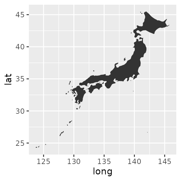
ggfortify additionally allows to autoplot map instances as it is. You can specify geom and other options to controll the outlooks.
## [1] "map"
autoplot(jp)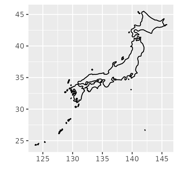
Also, maps package provides some geospatial data. Following example retrieves Japanese city locations from world’s city locations. Then plot on the previous map.
##         name country.etc    pop   lat   long capital
## 189 Abashiri       Japan  42324 44.02 144.27       0
## 221    Abiko       Japan 132577 35.88 140.03       0
## 481     Ageo       Japan 220766 35.95 139.61       0
## 514      Ago       Japan  23876 34.33 136.82       0
## 571     Agui       Japan  24227 34.95 136.91       0
## 629   Aikawa       Japan  43599 35.55 139.29       0
p + geom_point(data = cities, aes(x = long, y = lat),
               colour = 'blue', size = 0.1)
Because map plot created by ggfortify has a setting of aes(x = long, y = lat), you don’t have to specify x and y aethetics in this case.
p + geom_point(data = cities, colour = 'blue', size = 0.1)
Plotting with {sp} package
Also, ggfortify can supports geospatial instances defined in sp package. Actually some functions are defined in ggplot2. Following table shows where each function is defined.
| class | fortify |
autoplot |
|---|---|---|
Line |
ggplot2 | ggfortify |
Lines |
ggplot2 | ggfortify |
Polygon |
ggplot2 | ggfortify |
Polygons |
ggplot2 | ggfortify |
SpatialLines |
ggfortify | ggfortify |
SpatialLinesDataFrame |
ggplot2 | ggfortify |
SpatialPoints |
ggfortify | ggfortify |
SpatialPointsDataFrame |
ggfortify | ggfortify |
SpatialPolygons |
ggplot2 | ggfortify |
SpatialPolygonsDataFrame |
ggplot2 | ggfortify |
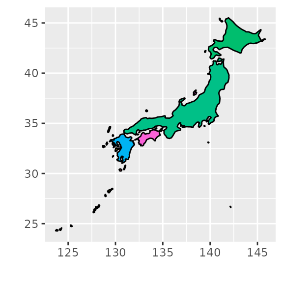
Following example creates SpatialPointsDataFrame of some Japanese city’s populatios, then plot it via autoplot. Note that you geom is specified by the original sp class. SpatialPoints is plot using geom_point for example.
library(sp)
df <- data.frame(long = c(139.691704, 135.519711),
                 lat = c(35.689521, 34.686316),
                 label = c('Tokyo', 'Osaka'),
                 population = c(1335, 886))
coordinates(df) <- ~ long + lat
class(df)
## [1] "SpatialPointsDataFrame"
## attr(,"package")
## [1] "sp"
autoplot(df, p = p, colour = 'red', size = 10)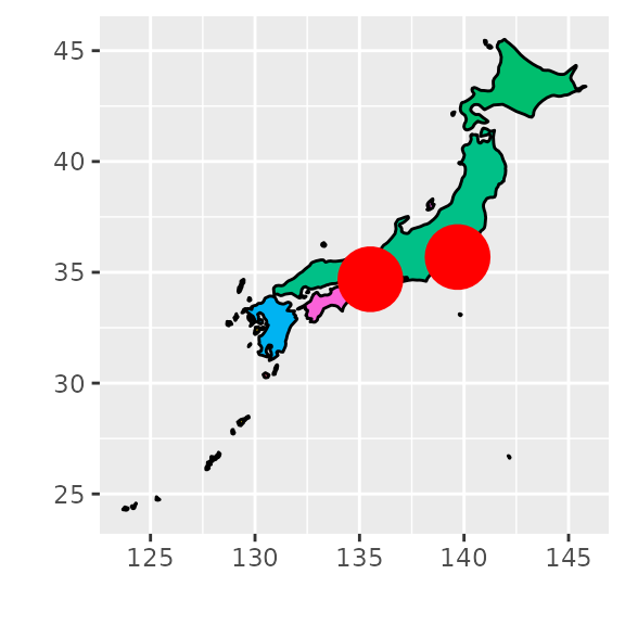
Also, you can use other columns as aethetics.
autoplot(df, p = p, colour = 'red', size = 'population') +
  scale_size_area()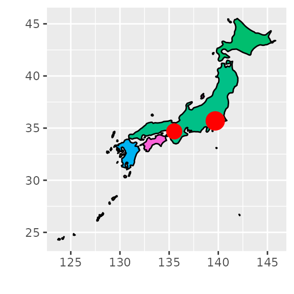
Plotting with other packages
autoplot has p keyword to take existing ggplot instance. Below example plots SpatialPointsDataFrame on the ggmap.
library(ggmap)
bbox <- c(130.0, 30.0, 145.0, 45.0)
map <- get_openstreetmap(bbox = bbox, scale = 47500000)
p <- ggmap(map)
autoplot(df, p = p, colour = 'red', size = 'population') +
  scale_size_area() +
  theme(legend.justification = c(1, 0), legend.position = c(1, 0))
ggmap_output