Basis dimension choice for smooths
choose.k.RdChoosing the basis dimension, and checking the choice, when using penalized regression smoothers.
Penalized regression smoothers gain computational efficiency by virtue of
being defined using a basis of relatively modest size, k. When setting
up models in the mgcv package, using s or te
terms in a model formula, k must be chosen: the defaults are essentially arbitrary.
In practice k-1 (or k) sets the upper limit on the degrees of freedom
associated with an s smooth (1 degree of freedom is usually lost to the identifiability
constraint on the smooth). For te smooths the upper limit of the
degrees of freedom is given by the product of the k values provided for
each marginal smooth less one, for the constraint. However the actual
effective degrees of freedom are controlled by the degree of penalization
selected during fitting, by GCV, AIC, REML or whatever is specified. The exception
to this is if a smooth is specified using the fx=TRUE option, in which
case it is unpenalized.
So, exact choice of k is not generally critical: it should be chosen to
be large enough that you are reasonably sure of having enough degrees of
freedom to represent the underlying `truth' reasonably well, but small enough
to maintain reasonable computational efficiency. Clearly `large' and `small'
are dependent on the particular problem being addressed.
As with all model assumptions, it is useful to be able to check the choice of
k informally. If the effective degrees of freedom for a model term are
estimated to be much less than k-1 then this is unlikely to be very
worthwhile, but as the EDF approach k-1, checking can be important. A
useful general purpose approach goes as follows: (i) fit your model and
extract the deviance residuals; (ii) for each smooth term in your model, fit
an equivalent, single, smooth to the residuals, using a substantially
increased k to see if there is pattern in the residuals that could
potentially be explained by increasing k. Examples are provided below.
The obvious, but more costly, alternative is simply to increase the suspect k
and refit the original model. If there are no statistically important changes as a result of
doing this, then k was large enough. (Change in the smoothness selection criterion,
and/or the effective degrees of freedom, when k is increased, provide the obvious
numerical measures for whether the fit has changed substantially.)
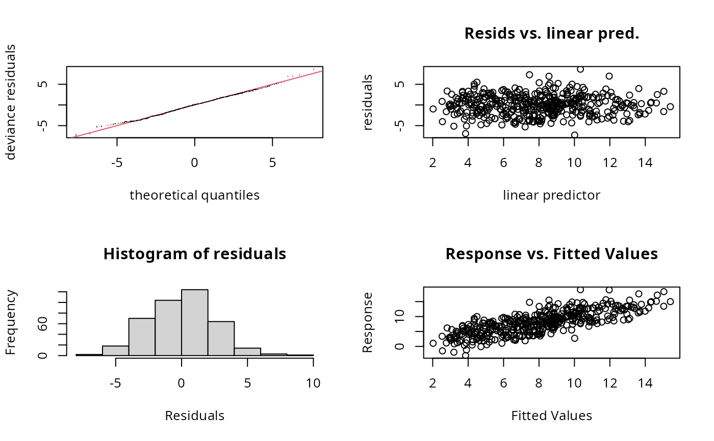
gam.check runs a simple simulation based check on the basis dimensions, which can
help to flag up terms for which k is too low. Grossly too small k
will also be visible from partial residuals available with plot.gam.
One scenario that can cause confusion is this: a model is fitted with
k=10 for a smooth term, and the EDF for the term is estimated as 7.6,
some way below the maximum of 9. The model is then refitted with k=20
and the EDF increases to 8.7 - what is happening - how come the EDF was not
8.7 the first time around? The explanation is that the function space with
k=20 contains a larger subspace of functions with EDF 8.7 than did the
function space with k=10: one of the functions in this larger subspace
fits the data a little better than did any function in the smaller
subspace. These subtleties seldom have much impact on the statistical
conclusions to be drawn from a model fit, however.
References
Wood, S.N. (2017) Generalized Additive Models: An Introduction with R (2nd edition). CRC/Taylor & Francis.
Examples
## Simulate some data ....
library(mgcv)
set.seed(1)
dat <- gamSim(1,n=400,scale=2)
#> Gu & Wahba 4 term additive model
## fit a GAM with quite low `k'
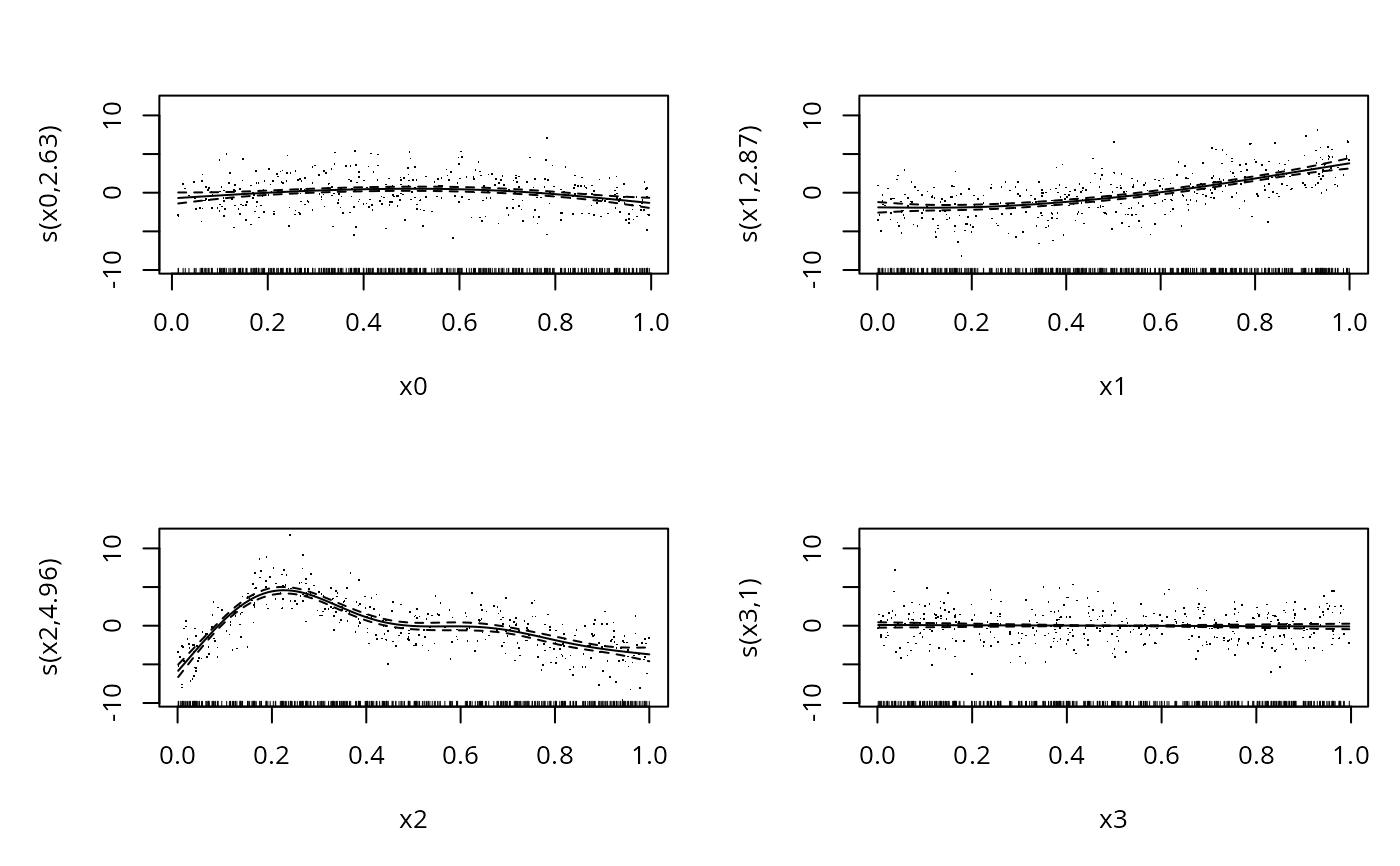
b<-gam(y~s(x0,k=6)+s(x1,k=6)+s(x2,k=6)+s(x3,k=6),data=dat)
plot(b,pages=1,residuals=TRUE) ## hint of a problem in s(x2)
 ## the following suggests a problem with s(x2)
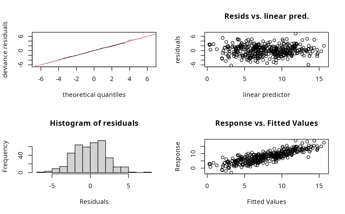
gam.check(b)
## the following suggests a problem with s(x2)
gam.check(b)
 #>
#> Method: GCV Optimizer: magic
#> Smoothing parameter selection converged after 17 iterations.
#> The RMS GCV score gradient at convergence was 2.675921e-07 .
#> The Hessian was positive definite.
#> Model rank = 21 / 21
#>
#> Basis dimension (k) checking results. Low p-value (k-index<1) may
#> indicate that k is too low, especially if edf is close to k'.
#>
#> k' edf k-index p-value
#> s(x0) 5.00 2.63 0.98 0.260
#> s(x1) 5.00 2.87 0.99 0.405
#> s(x2) 5.00 4.96 0.92 0.065 .
#> s(x3) 5.00 1.00 1.02 0.660
#> ---
#> Signif. codes: 0 ‘***’ 0.001 ‘**’ 0.01 ‘*’ 0.05 ‘.’ 0.1 ‘ ’ 1
## Another approach (see below for more obvious method)....
## check for residual pattern, removeable by increasing `k'
## typically `k', below, chould be substantially larger than
## the original, `k' but certainly less than n/2.
## Note use of cheap "cs" shrinkage smoothers, and gamma=1.4
## to reduce chance of overfitting...
rsd <- residuals(b)
gam(rsd~s(x0,k=40,bs="cs"),gamma=1.4,data=dat) ## fine
#>
#> Family: gaussian
#> Link function: identity
#>
#> Formula:
#> rsd ~ s(x0, k = 40, bs = "cs")
#>
#> Estimated degrees of freedom:
#> 0 total = 1
#>
#> GCV score: 4.448352
gam(rsd~s(x1,k=40,bs="cs"),gamma=1.4,data=dat) ## fine
#>
#> Family: gaussian
#> Link function: identity
#>
#> Formula:
#> rsd ~ s(x1, k = 40, bs = "cs")
#>
#> Estimated degrees of freedom:
#> 0 total = 1
#>
#> GCV score: 4.448352
gam(rsd~s(x2,k=40,bs="cs"),gamma=1.4,data=dat) ## `k' too low
#>
#> Family: gaussian
#> Link function: identity
#>
#> Formula:
#> rsd ~ s(x2, k = 40, bs = "cs")
#>
#> Estimated degrees of freedom:
#> 9.01 total = 10.01
#>
#> GCV score: 4.494652
gam(rsd~s(x3,k=40,bs="cs"),gamma=1.4,data=dat) ## fine
#>
#> Family: gaussian
#> Link function: identity
#>
#> Formula:
#> rsd ~ s(x3, k = 40, bs = "cs")
#>
#> Estimated degrees of freedom:
#> 0 total = 1
#>
#> GCV score: 4.448352
## refit...
b <- gam(y~s(x0,k=6)+s(x1,k=6)+s(x2,k=20)+s(x3,k=6),data=dat)
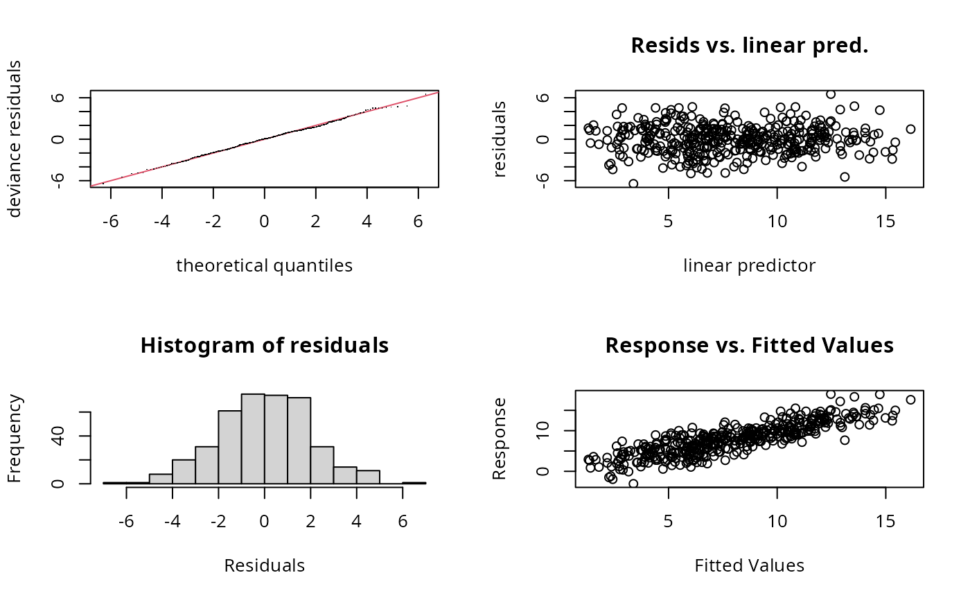
gam.check(b) ## better
#>
#> Method: GCV Optimizer: magic
#> Smoothing parameter selection converged after 17 iterations.
#> The RMS GCV score gradient at convergence was 2.675921e-07 .
#> The Hessian was positive definite.
#> Model rank = 21 / 21
#>
#> Basis dimension (k) checking results. Low p-value (k-index<1) may
#> indicate that k is too low, especially if edf is close to k'.
#>
#> k' edf k-index p-value
#> s(x0) 5.00 2.63 0.98 0.260
#> s(x1) 5.00 2.87 0.99 0.405
#> s(x2) 5.00 4.96 0.92 0.065 .
#> s(x3) 5.00 1.00 1.02 0.660
#> ---
#> Signif. codes: 0 ‘***’ 0.001 ‘**’ 0.01 ‘*’ 0.05 ‘.’ 0.1 ‘ ’ 1
## Another approach (see below for more obvious method)....
## check for residual pattern, removeable by increasing `k'
## typically `k', below, chould be substantially larger than
## the original, `k' but certainly less than n/2.
## Note use of cheap "cs" shrinkage smoothers, and gamma=1.4
## to reduce chance of overfitting...
rsd <- residuals(b)
gam(rsd~s(x0,k=40,bs="cs"),gamma=1.4,data=dat) ## fine
#>
#> Family: gaussian
#> Link function: identity
#>
#> Formula:
#> rsd ~ s(x0, k = 40, bs = "cs")
#>
#> Estimated degrees of freedom:
#> 0 total = 1
#>
#> GCV score: 4.448352
gam(rsd~s(x1,k=40,bs="cs"),gamma=1.4,data=dat) ## fine
#>
#> Family: gaussian
#> Link function: identity
#>
#> Formula:
#> rsd ~ s(x1, k = 40, bs = "cs")
#>
#> Estimated degrees of freedom:
#> 0 total = 1
#>
#> GCV score: 4.448352
gam(rsd~s(x2,k=40,bs="cs"),gamma=1.4,data=dat) ## `k' too low
#>
#> Family: gaussian
#> Link function: identity
#>
#> Formula:
#> rsd ~ s(x2, k = 40, bs = "cs")
#>
#> Estimated degrees of freedom:
#> 9.01 total = 10.01
#>
#> GCV score: 4.494652
gam(rsd~s(x3,k=40,bs="cs"),gamma=1.4,data=dat) ## fine
#>
#> Family: gaussian
#> Link function: identity
#>
#> Formula:
#> rsd ~ s(x3, k = 40, bs = "cs")
#>
#> Estimated degrees of freedom:
#> 0 total = 1
#>
#> GCV score: 4.448352
## refit...
b <- gam(y~s(x0,k=6)+s(x1,k=6)+s(x2,k=20)+s(x3,k=6),data=dat)
gam.check(b) ## better
 #>
#> Method: GCV Optimizer: magic
#> Smoothing parameter selection converged after 9 iterations.
#> The RMS GCV score gradient at convergence was 2.918624e-07 .
#> The Hessian was positive definite.
#> Model rank = 35 / 35
#>
#> Basis dimension (k) checking results. Low p-value (k-index<1) may
#> indicate that k is too low, especially if edf is close to k'.
#>
#> k' edf k-index p-value
#> s(x0) 5.00 2.70 0.98 0.37
#> s(x1) 5.00 2.62 0.98 0.33
#> s(x2) 19.00 11.22 0.98 0.37
#> s(x3) 5.00 1.00 1.02 0.70
## similar example with multi-dimensional smooth
b1 <- gam(y~s(x0)+s(x1,x2,k=15)+s(x3),data=dat)
rsd <- residuals(b1)
gam(rsd~s(x0,k=40,bs="cs"),gamma=1.4,data=dat) ## fine
#>
#> Family: gaussian
#> Link function: identity
#>
#> Formula:
#> rsd ~ s(x0, k = 40, bs = "cs")
#>
#> Estimated degrees of freedom:
#> 0 total = 1
#>
#> GCV score: 5.257725
gam(rsd~s(x1,x2,k=100,bs="ts"),gamma=1.4,data=dat) ## `k' too low
#>
#> Family: gaussian
#> Link function: identity
#>
#> Formula:
#> rsd ~ s(x1, x2, k = 100, bs = "ts")
#>
#> Estimated degrees of freedom:
#> 30.6 total = 31.62
#>
#> GCV score: 5.066268
gam(rsd~s(x3,k=40,bs="cs"),gamma=1.4,data=dat) ## fine
#>
#> Family: gaussian
#> Link function: identity
#>
#> Formula:
#> rsd ~ s(x3, k = 40, bs = "cs")
#>
#> Estimated degrees of freedom:
#> 0 total = 1
#>
#> GCV score: 5.257725
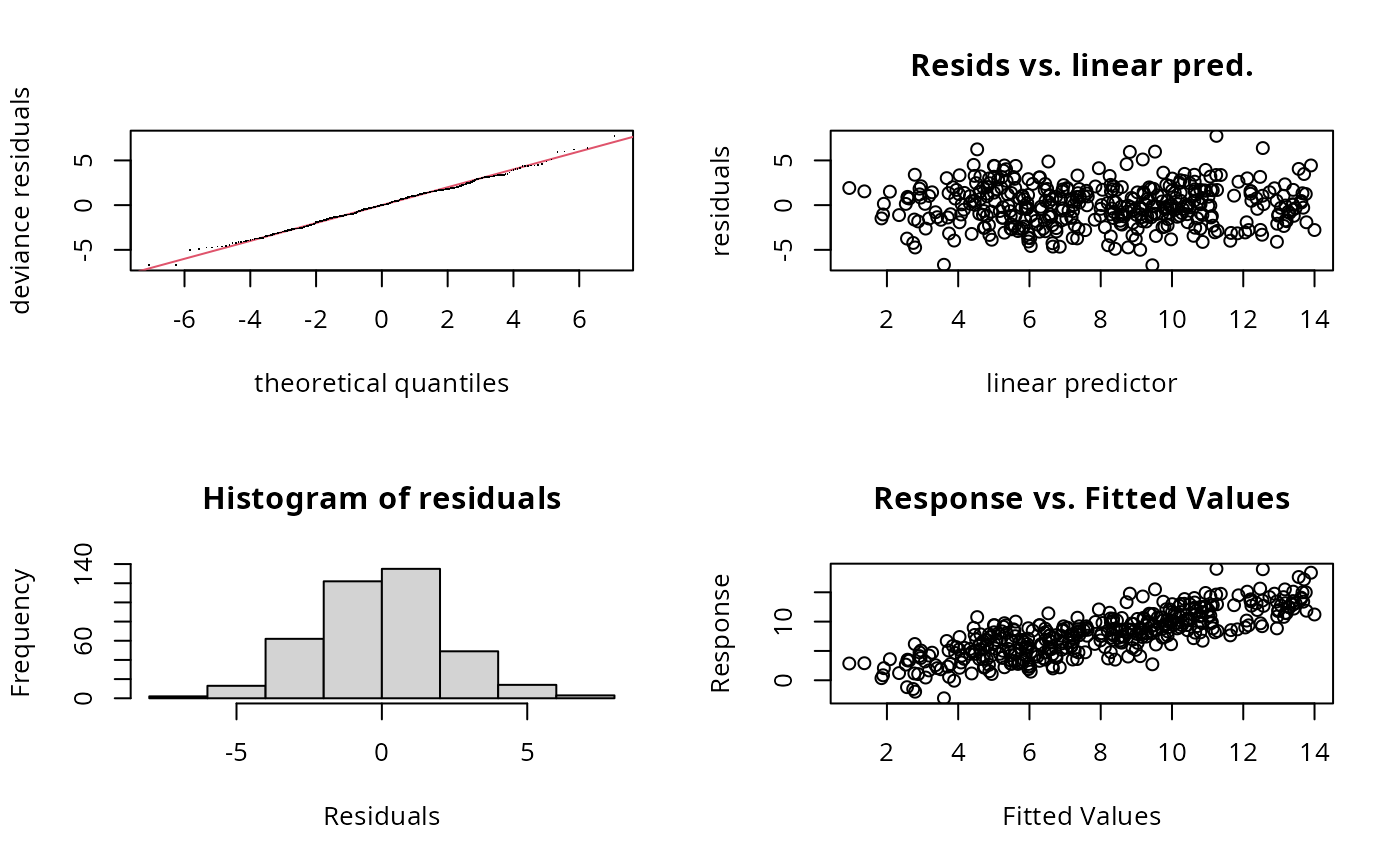
gam.check(b1) ## shows same problem
#>
#> Method: GCV Optimizer: magic
#> Smoothing parameter selection converged after 9 iterations.
#> The RMS GCV score gradient at convergence was 2.918624e-07 .
#> The Hessian was positive definite.
#> Model rank = 35 / 35
#>
#> Basis dimension (k) checking results. Low p-value (k-index<1) may
#> indicate that k is too low, especially if edf is close to k'.
#>
#> k' edf k-index p-value
#> s(x0) 5.00 2.70 0.98 0.37
#> s(x1) 5.00 2.62 0.98 0.33
#> s(x2) 19.00 11.22 0.98 0.37
#> s(x3) 5.00 1.00 1.02 0.70
## similar example with multi-dimensional smooth
b1 <- gam(y~s(x0)+s(x1,x2,k=15)+s(x3),data=dat)
rsd <- residuals(b1)
gam(rsd~s(x0,k=40,bs="cs"),gamma=1.4,data=dat) ## fine
#>
#> Family: gaussian
#> Link function: identity
#>
#> Formula:
#> rsd ~ s(x0, k = 40, bs = "cs")
#>
#> Estimated degrees of freedom:
#> 0 total = 1
#>
#> GCV score: 5.257725
gam(rsd~s(x1,x2,k=100,bs="ts"),gamma=1.4,data=dat) ## `k' too low
#>
#> Family: gaussian
#> Link function: identity
#>
#> Formula:
#> rsd ~ s(x1, x2, k = 100, bs = "ts")
#>
#> Estimated degrees of freedom:
#> 30.6 total = 31.62
#>
#> GCV score: 5.066268
gam(rsd~s(x3,k=40,bs="cs"),gamma=1.4,data=dat) ## fine
#>
#> Family: gaussian
#> Link function: identity
#>
#> Formula:
#> rsd ~ s(x3, k = 40, bs = "cs")
#>
#> Estimated degrees of freedom:
#> 0 total = 1
#>
#> GCV score: 5.257725
gam.check(b1) ## shows same problem
 #>
#> Method: GCV Optimizer: magic
#> Smoothing parameter selection converged after 15 iterations.
#> The RMS GCV score gradient at convergence was 2.956997e-07 .
#> The Hessian was positive definite.
#> Model rank = 33 / 33
#>
#> Basis dimension (k) checking results. Low p-value (k-index<1) may
#> indicate that k is too low, especially if edf is close to k'.
#>
#> k' edf k-index p-value
#> s(x0) 9.00 2.46 0.97 0.18
#> s(x1,x2) 14.00 13.74 0.83 <2e-16 ***
#> s(x3) 9.00 1.00 1.00 0.47
#> ---
#> Signif. codes: 0 ‘***’ 0.001 ‘**’ 0.01 ‘*’ 0.05 ‘.’ 0.1 ‘ ’ 1
## and a `te' example
b2 <- gam(y~s(x0)+te(x1,x2,k=4)+s(x3),data=dat)
rsd <- residuals(b2)
gam(rsd~s(x0,k=40,bs="cs"),gamma=1.4,data=dat) ## fine
#>
#> Family: gaussian
#> Link function: identity
#>
#> Formula:
#> rsd ~ s(x0, k = 40, bs = "cs")
#>
#> Estimated degrees of freedom:
#> 0 total = 1
#>
#> GCV score: 6.181669
gam(rsd~te(x1,x2,k=10,bs="cs"),gamma=1.4,data=dat) ## `k' too low
#>
#> Family: gaussian
#> Link function: identity
#>
#> Formula:
#> rsd ~ te(x1, x2, k = 10, bs = "cs")
#>
#> Estimated degrees of freedom:
#> 17 total = 18.05
#>
#> GCV score: 4.565293
gam(rsd~s(x3,k=40,bs="cs"),gamma=1.4,data=dat) ## fine
#>
#> Family: gaussian
#> Link function: identity
#>
#> Formula:
#> rsd ~ s(x3, k = 40, bs = "cs")
#>
#> Estimated degrees of freedom:
#> 0 total = 1
#>
#> GCV score: 6.181669
gam.check(b2) ## shows same problem
#>
#> Method: GCV Optimizer: magic
#> Smoothing parameter selection converged after 15 iterations.
#> The RMS GCV score gradient at convergence was 2.956997e-07 .
#> The Hessian was positive definite.
#> Model rank = 33 / 33
#>
#> Basis dimension (k) checking results. Low p-value (k-index<1) may
#> indicate that k is too low, especially if edf is close to k'.
#>
#> k' edf k-index p-value
#> s(x0) 9.00 2.46 0.97 0.18
#> s(x1,x2) 14.00 13.74 0.83 <2e-16 ***
#> s(x3) 9.00 1.00 1.00 0.47
#> ---
#> Signif. codes: 0 ‘***’ 0.001 ‘**’ 0.01 ‘*’ 0.05 ‘.’ 0.1 ‘ ’ 1
## and a `te' example
b2 <- gam(y~s(x0)+te(x1,x2,k=4)+s(x3),data=dat)
rsd <- residuals(b2)
gam(rsd~s(x0,k=40,bs="cs"),gamma=1.4,data=dat) ## fine
#>
#> Family: gaussian
#> Link function: identity
#>
#> Formula:
#> rsd ~ s(x0, k = 40, bs = "cs")
#>
#> Estimated degrees of freedom:
#> 0 total = 1
#>
#> GCV score: 6.181669
gam(rsd~te(x1,x2,k=10,bs="cs"),gamma=1.4,data=dat) ## `k' too low
#>
#> Family: gaussian
#> Link function: identity
#>
#> Formula:
#> rsd ~ te(x1, x2, k = 10, bs = "cs")
#>
#> Estimated degrees of freedom:
#> 17 total = 18.05
#>
#> GCV score: 4.565293
gam(rsd~s(x3,k=40,bs="cs"),gamma=1.4,data=dat) ## fine
#>
#> Family: gaussian
#> Link function: identity
#>
#> Formula:
#> rsd ~ s(x3, k = 40, bs = "cs")
#>
#> Estimated degrees of freedom:
#> 0 total = 1
#>
#> GCV score: 6.181669
gam.check(b2) ## shows same problem
 #>
#> Method: GCV Optimizer: magic
#> Smoothing parameter selection converged after 15 iterations.
#> The RMS GCV score gradient at convergence was 2.875373e-07 .
#> The Hessian was positive definite.
#> Model rank = 34 / 34
#>
#> Basis dimension (k) checking results. Low p-value (k-index<1) may
#> indicate that k is too low, especially if edf is close to k'.
#>
#> k' edf k-index p-value
#> s(x0) 9.00 2.60 1.05 0.83
#> te(x1,x2) 15.00 9.94 0.68 <2e-16 ***
#> s(x3) 9.00 1.00 0.96 0.18
#> ---
#> Signif. codes: 0 ‘***’ 0.001 ‘**’ 0.01 ‘*’ 0.05 ‘.’ 0.1 ‘ ’ 1
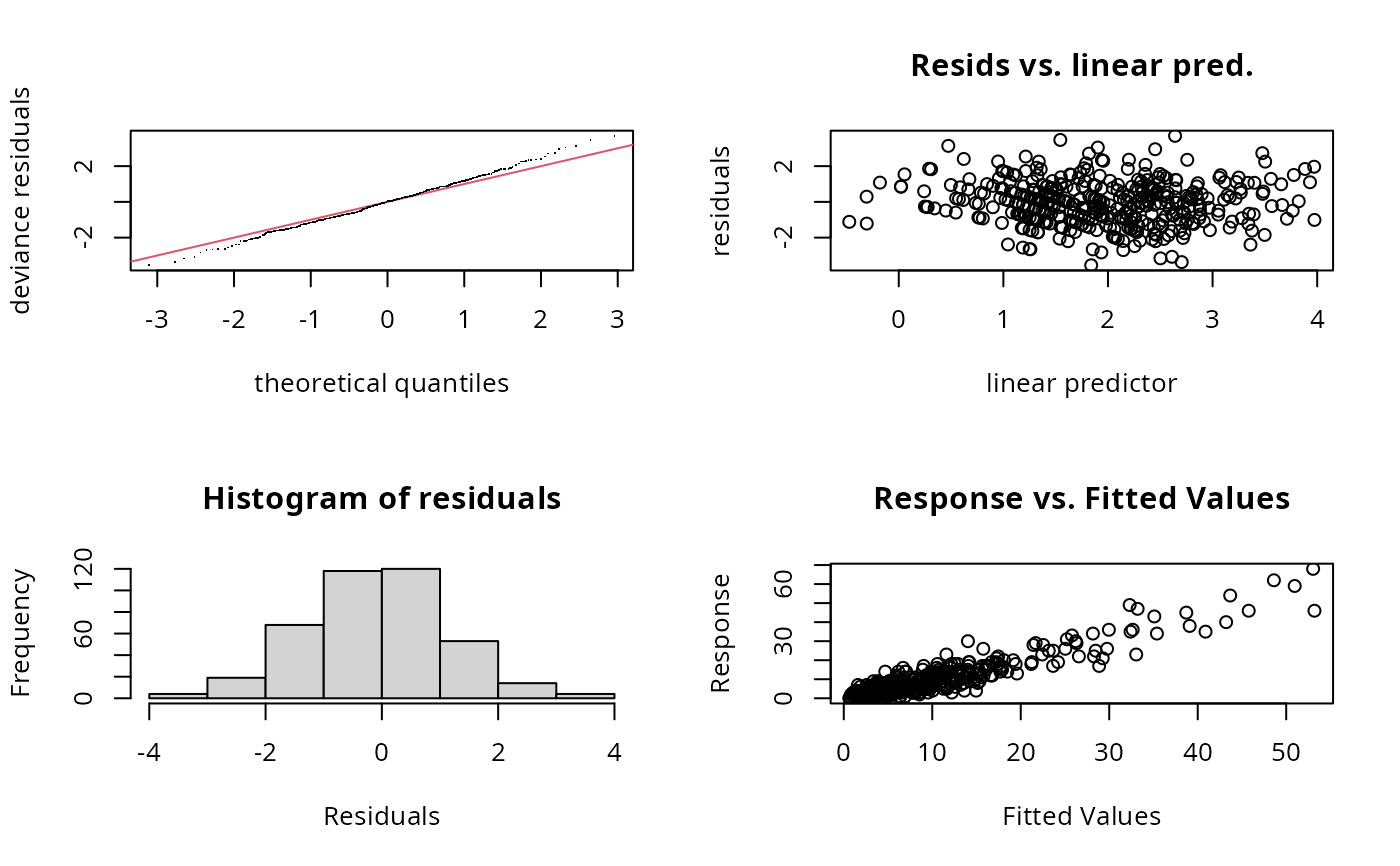
## same approach works with other families in the original model
dat <- gamSim(1,n=400,scale=.25,dist="poisson")
#> Gu & Wahba 4 term additive model
bp<-gam(y~s(x0,k=5)+s(x1,k=5)+s(x2,k=5)+s(x3,k=5),
family=poisson,data=dat,method="ML")
gam.check(bp)
#>
#> Method: GCV Optimizer: magic
#> Smoothing parameter selection converged after 15 iterations.
#> The RMS GCV score gradient at convergence was 2.875373e-07 .
#> The Hessian was positive definite.
#> Model rank = 34 / 34
#>
#> Basis dimension (k) checking results. Low p-value (k-index<1) may
#> indicate that k is too low, especially if edf is close to k'.
#>
#> k' edf k-index p-value
#> s(x0) 9.00 2.60 1.05 0.83
#> te(x1,x2) 15.00 9.94 0.68 <2e-16 ***
#> s(x3) 9.00 1.00 0.96 0.18
#> ---
#> Signif. codes: 0 ‘***’ 0.001 ‘**’ 0.01 ‘*’ 0.05 ‘.’ 0.1 ‘ ’ 1
## same approach works with other families in the original model
dat <- gamSim(1,n=400,scale=.25,dist="poisson")
#> Gu & Wahba 4 term additive model
bp<-gam(y~s(x0,k=5)+s(x1,k=5)+s(x2,k=5)+s(x3,k=5),
family=poisson,data=dat,method="ML")
gam.check(bp)
 #>
#> Method: ML Optimizer: outer newton
#> full convergence after 9 iterations.
#> Gradient range [-0.0001745332,1.193507e-06]
#> (score 1063.418 & scale 1).
#> Hessian positive definite, eigenvalue range [0.0001744834,1.4833].
#> Model rank = 17 / 17
#>
#> Basis dimension (k) checking results. Low p-value (k-index<1) may
#> indicate that k is too low, especially if edf is close to k'.
#>
#> k' edf k-index p-value
#> s(x0) 4.00 3.37 1.00 0.57
#> s(x1) 4.00 3.01 1.02 0.63
#> s(x2) 4.00 3.99 0.73 <2e-16 ***
#> s(x3) 4.00 1.00 0.98 0.34
#> ---
#> Signif. codes: 0 ‘***’ 0.001 ‘**’ 0.01 ‘*’ 0.05 ‘.’ 0.1 ‘ ’ 1
rsd <- residuals(bp)
gam(rsd~s(x0,k=40,bs="cs"),gamma=1.4,data=dat) ## fine
#>
#> Family: gaussian
#> Link function: identity
#>
#> Formula:
#> rsd ~ s(x0, k = 40, bs = "cs")
#>
#> Estimated degrees of freedom:
#> 0 total = 1
#>
#> GCV score: 1.504487
gam(rsd~s(x1,k=40,bs="cs"),gamma=1.4,data=dat) ## fine
#>
#> Family: gaussian
#> Link function: identity
#>
#> Formula:
#> rsd ~ s(x1, k = 40, bs = "cs")
#>
#> Estimated degrees of freedom:
#> 0 total = 1
#>
#> GCV score: 1.504487
gam(rsd~s(x2,k=40,bs="cs"),gamma=1.4,data=dat) ## `k' too low
#>
#> Family: gaussian
#> Link function: identity
#>
#> Formula:
#> rsd ~ s(x2, k = 40, bs = "cs")
#>
#> Estimated degrees of freedom:
#> 10.9 total = 11.85
#>
#> GCV score: 1.141074
gam(rsd~s(x3,k=40,bs="cs"),gamma=1.4,data=dat) ## fine
#>
#> Family: gaussian
#> Link function: identity
#>
#> Formula:
#> rsd ~ s(x3, k = 40, bs = "cs")
#>
#> Estimated degrees of freedom:
#> 3.79 total = 4.79
#>
#> GCV score: 1.515055
rm(dat)
## More obvious, but more expensive tactic... Just increase
## suspicious k until fit is stable.
set.seed(0)
dat <- gamSim(1,n=400,scale=2)
#> Gu & Wahba 4 term additive model
## fit a GAM with quite low `k'
b <- gam(y~s(x0,k=6)+s(x1,k=6)+s(x2,k=6)+s(x3,k=6),
data=dat,method="REML")
b
#>
#> Family: gaussian
#> Link function: identity
#>
#> Formula:
#> y ~ s(x0, k = 6) + s(x1, k = 6) + s(x2, k = 6) + s(x3, k = 6)
#>
#> Estimated degrees of freedom:
#> 2.90 2.71 4.94 1.00 total = 12.55
#>
#> REML score: 892.3014
## edf for 3rd smooth is highest as proportion of k -- increase k
b <- gam(y~s(x0,k=6)+s(x1,k=6)+s(x2,k=12)+s(x3,k=6),
data=dat,method="REML")
b
#>
#> Family: gaussian
#> Link function: identity
#>
#> Formula:
#> y ~ s(x0, k = 6) + s(x1, k = 6) + s(x2, k = 12) + s(x3, k = 6)
#>
#> Estimated degrees of freedom:
#> 3.10 2.67 9.07 1.00 total = 16.84
#>
#> REML score: 887.9842
## edf substantially up, -ve REML substantially down
b <- gam(y~s(x0,k=6)+s(x1,k=6)+s(x2,k=24)+s(x3,k=6),
data=dat,method="REML")
b
#>
#> Family: gaussian
#> Link function: identity
#>
#> Formula:
#> y ~ s(x0, k = 6) + s(x1, k = 6) + s(x2, k = 24) + s(x3, k = 6)
#>
#> Estimated degrees of freedom:
#> 3.12 2.67 11.32 1.00 total = 19.11
#>
#> REML score: 887.0976
## slight edf increase and -ve REML change
b <- gam(y~s(x0,k=6)+s(x1,k=6)+s(x2,k=40)+s(x3,k=6),
data=dat,method="REML")
b
#>
#> Family: gaussian
#> Link function: identity
#>
#> Formula:
#> y ~ s(x0, k = 6) + s(x1, k = 6) + s(x2, k = 40) + s(x3, k = 6)
#>
#> Estimated degrees of freedom:
#> 3.12 2.67 11.54 1.00 total = 19.33
#>
#> REML score: 887.1258
## defintely stabilized (but really k around 20 would have been fine)
#>
#> Method: ML Optimizer: outer newton
#> full convergence after 9 iterations.
#> Gradient range [-0.0001745332,1.193507e-06]
#> (score 1063.418 & scale 1).
#> Hessian positive definite, eigenvalue range [0.0001744834,1.4833].
#> Model rank = 17 / 17
#>
#> Basis dimension (k) checking results. Low p-value (k-index<1) may
#> indicate that k is too low, especially if edf is close to k'.
#>
#> k' edf k-index p-value
#> s(x0) 4.00 3.37 1.00 0.57
#> s(x1) 4.00 3.01 1.02 0.63
#> s(x2) 4.00 3.99 0.73 <2e-16 ***
#> s(x3) 4.00 1.00 0.98 0.34
#> ---
#> Signif. codes: 0 ‘***’ 0.001 ‘**’ 0.01 ‘*’ 0.05 ‘.’ 0.1 ‘ ’ 1
rsd <- residuals(bp)
gam(rsd~s(x0,k=40,bs="cs"),gamma=1.4,data=dat) ## fine
#>
#> Family: gaussian
#> Link function: identity
#>
#> Formula:
#> rsd ~ s(x0, k = 40, bs = "cs")
#>
#> Estimated degrees of freedom:
#> 0 total = 1
#>
#> GCV score: 1.504487
gam(rsd~s(x1,k=40,bs="cs"),gamma=1.4,data=dat) ## fine
#>
#> Family: gaussian
#> Link function: identity
#>
#> Formula:
#> rsd ~ s(x1, k = 40, bs = "cs")
#>
#> Estimated degrees of freedom:
#> 0 total = 1
#>
#> GCV score: 1.504487
gam(rsd~s(x2,k=40,bs="cs"),gamma=1.4,data=dat) ## `k' too low
#>
#> Family: gaussian
#> Link function: identity
#>
#> Formula:
#> rsd ~ s(x2, k = 40, bs = "cs")
#>
#> Estimated degrees of freedom:
#> 10.9 total = 11.85
#>
#> GCV score: 1.141074
gam(rsd~s(x3,k=40,bs="cs"),gamma=1.4,data=dat) ## fine
#>
#> Family: gaussian
#> Link function: identity
#>
#> Formula:
#> rsd ~ s(x3, k = 40, bs = "cs")
#>
#> Estimated degrees of freedom:
#> 3.79 total = 4.79
#>
#> GCV score: 1.515055
rm(dat)
## More obvious, but more expensive tactic... Just increase
## suspicious k until fit is stable.
set.seed(0)
dat <- gamSim(1,n=400,scale=2)
#> Gu & Wahba 4 term additive model
## fit a GAM with quite low `k'
b <- gam(y~s(x0,k=6)+s(x1,k=6)+s(x2,k=6)+s(x3,k=6),
data=dat,method="REML")
b
#>
#> Family: gaussian
#> Link function: identity
#>
#> Formula:
#> y ~ s(x0, k = 6) + s(x1, k = 6) + s(x2, k = 6) + s(x3, k = 6)
#>
#> Estimated degrees of freedom:
#> 2.90 2.71 4.94 1.00 total = 12.55
#>
#> REML score: 892.3014
## edf for 3rd smooth is highest as proportion of k -- increase k
b <- gam(y~s(x0,k=6)+s(x1,k=6)+s(x2,k=12)+s(x3,k=6),
data=dat,method="REML")
b
#>
#> Family: gaussian
#> Link function: identity
#>
#> Formula:
#> y ~ s(x0, k = 6) + s(x1, k = 6) + s(x2, k = 12) + s(x3, k = 6)
#>
#> Estimated degrees of freedom:
#> 3.10 2.67 9.07 1.00 total = 16.84
#>
#> REML score: 887.9842
## edf substantially up, -ve REML substantially down
b <- gam(y~s(x0,k=6)+s(x1,k=6)+s(x2,k=24)+s(x3,k=6),
data=dat,method="REML")
b
#>
#> Family: gaussian
#> Link function: identity
#>
#> Formula:
#> y ~ s(x0, k = 6) + s(x1, k = 6) + s(x2, k = 24) + s(x3, k = 6)
#>
#> Estimated degrees of freedom:
#> 3.12 2.67 11.32 1.00 total = 19.11
#>
#> REML score: 887.0976
## slight edf increase and -ve REML change
b <- gam(y~s(x0,k=6)+s(x1,k=6)+s(x2,k=40)+s(x3,k=6),
data=dat,method="REML")
b
#>
#> Family: gaussian
#> Link function: identity
#>
#> Formula:
#> y ~ s(x0, k = 6) + s(x1, k = 6) + s(x2, k = 40) + s(x3, k = 6)
#>
#> Estimated degrees of freedom:
#> 3.12 2.67 11.54 1.00 total = 19.33
#>
#> REML score: 887.1258
## defintely stabilized (but really k around 20 would have been fine)