Gamma location-scale model family
gammals.RdThe gammals family implements gamma location scale additive models in which
the log of the mean, \(\mu\), and the log of the scale parameter, \(\phi\) (see details) can depend on additive smooth predictors. The parameterization is of the usual GLM type where the variance of the response is given by \(\phi\mu^2\). Useable only with gam, the linear predictors are specified via a list of formulae.
gammals(link=list("identity","log"),b=-7)Arguments
Value
An object inheriting from class general.family.
Details
Used with gam to fit gamma location - scale models parameterized in terms of the log mean and the log scale parameter (the response variance is the squared mean multiplied by the scale parameter). Note that identity links mean that the linear predictors give the log mean and log scale directly. By default the log link for the scale parameter simply forces the log scale parameter to have a lower limit given by argument b: if \(\eta\) is the linear predictor for the log scale parameter, \(\phi\), then \(\log \phi = b + \log(1+e^{\eta-b})\).
gam is called with
a list containing 2 formulae, the first specifies the response on the left hand side and the structure of the linear predictor for the log mean on the right hand side. The second is one sided, specifying the linear predictor for the log scale on the right hand side.
The fitted values for this family will be a two column matrix. The first column is the mean (on original, not log, scale), and the second column is the log scale. Predictions using predict.gam will also produce 2 column matrices for type "link" and "response". The first column is on the original data scale when type="response" and on the log mean scale of the linear predictor when type="link". The second column when type="response" is again the log scale parameter, but is on the linear predictor when type="link".
The null deviance reported for this family computed by setting the fitted values to the mean response, but using the model estimated scale.
References
Wood, S.N., N. Pya and B. Saefken (2016), Smoothing parameter and model selection for general smooth models. Journal of the American Statistical Association 111, 1548-1575 doi:10.1080/01621459.2016.1180986
Examples
library(mgcv)
## simulate some data
f0 <- function(x) 2 * sin(pi * x)
f1 <- function(x) exp(2 * x)
f2 <- function(x) 0.2 * x^11 * (10 * (1 - x))^6 + 10 *
(10 * x)^3 * (1 - x)^10
f3 <- function(x) 0 * x
n <- 400;set.seed(9)
x0 <- runif(n);x1 <- runif(n);
x2 <- runif(n);x3 <- runif(n);
mu <- exp((f0(x0)+f2(x2))/5)
th <- exp(f1(x1)/2-2)
y <- rgamma(n,shape=1/th,scale=mu*th)
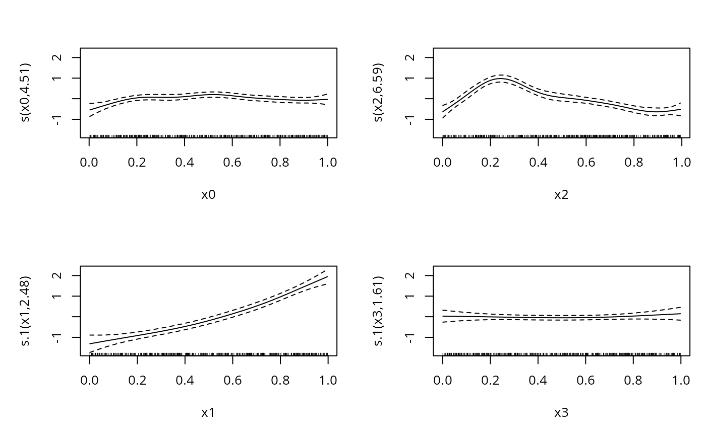
b1 <- gam(list(y~s(x0)+s(x2),~s(x1)+s(x3)),family=gammals)
plot(b1,pages=1)
 summary(b1)
#>
#> Family: gammals
#> Link function: identity log
#>
#> Formula:
#> y ~ s(x0) + s(x2)
#> <environment: 0x5efddfc753e8>
#> ~s(x1) + s(x3)
#> <environment: 0x5efddfc753e8>
#>
#> Parametric coefficients:
#> Estimate Std. Error z value Pr(>|z|)
#> (Intercept) 0.89430 0.03489 25.631 < 2e-16 ***
#> (Intercept).1 -0.39263 0.06466 -6.073 1.26e-09 ***
#> ---
#> Signif. codes: 0 ‘***’ 0.001 ‘**’ 0.01 ‘*’ 0.05 ‘.’ 0.1 ‘ ’ 1
#>
#> Approximate significance of smooth terms:
#> edf Ref.df Chi.sq p-value
#> s(x0) 4.510 5.512 17.918 0.00326 **
#> s(x2) 6.591 7.696 214.768 < 2e-16 ***
#> s.1(x1) 2.485 3.074 233.361 < 2e-16 ***
#> s.1(x3) 1.607 1.989 1.056 0.60225
#> ---
#> Signif. codes: 0 ‘***’ 0.001 ‘**’ 0.01 ‘*’ 0.05 ‘.’ 0.1 ‘ ’ 1
#>
#> Deviance explained = 36.4%
#> -REML = 655.32 Scale est. = 1 n = 400
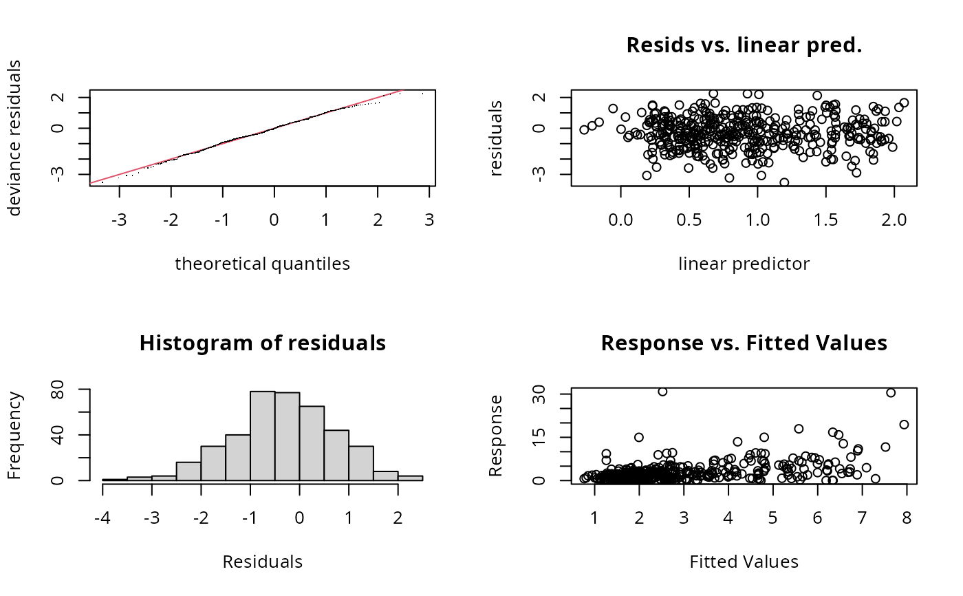
gam.check(b1)
summary(b1)
#>
#> Family: gammals
#> Link function: identity log
#>
#> Formula:
#> y ~ s(x0) + s(x2)
#> <environment: 0x5efddfc753e8>
#> ~s(x1) + s(x3)
#> <environment: 0x5efddfc753e8>
#>
#> Parametric coefficients:
#> Estimate Std. Error z value Pr(>|z|)
#> (Intercept) 0.89430 0.03489 25.631 < 2e-16 ***
#> (Intercept).1 -0.39263 0.06466 -6.073 1.26e-09 ***
#> ---
#> Signif. codes: 0 ‘***’ 0.001 ‘**’ 0.01 ‘*’ 0.05 ‘.’ 0.1 ‘ ’ 1
#>
#> Approximate significance of smooth terms:
#> edf Ref.df Chi.sq p-value
#> s(x0) 4.510 5.512 17.918 0.00326 **
#> s(x2) 6.591 7.696 214.768 < 2e-16 ***
#> s.1(x1) 2.485 3.074 233.361 < 2e-16 ***
#> s.1(x3) 1.607 1.989 1.056 0.60225
#> ---
#> Signif. codes: 0 ‘***’ 0.001 ‘**’ 0.01 ‘*’ 0.05 ‘.’ 0.1 ‘ ’ 1
#>
#> Deviance explained = 36.4%
#> -REML = 655.32 Scale est. = 1 n = 400
gam.check(b1)
 #>
#> Method: REML Optimizer: outer newton
#> full convergence after 5 iterations.
#> Gradient range [-0.0002211472,4.797707e-06]
#> (score 655.3212 & scale 1).
#> Hessian positive definite, eigenvalue range [0.08556541,2.116265].
#> Model rank = 38 / 38
#>
#> Basis dimension (k) checking results. Low p-value (k-index<1) may
#> indicate that k is too low, especially if edf is close to k'.
#>
#> k' edf k-index p-value
#> s(x0) 9.00 4.51 0.97 0.91
#> s(x2) 9.00 6.59 0.87 0.21
#> s.1(x1) 9.00 2.48 0.94 0.71
#> s.1(x3) 9.00 1.61 0.94 0.69
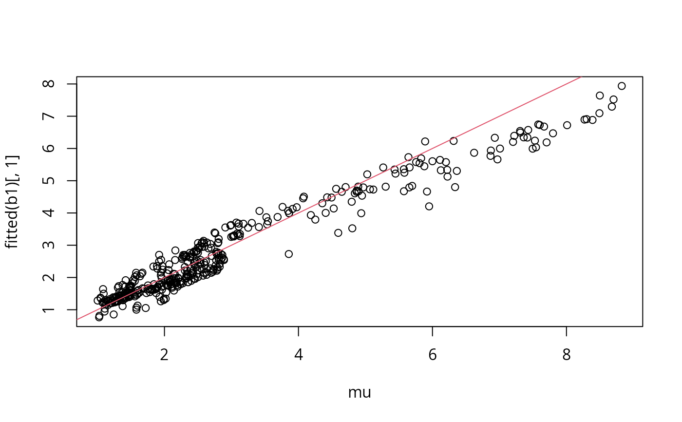
plot(mu,fitted(b1)[,1]);abline(0,1,col=2)
#>
#> Method: REML Optimizer: outer newton
#> full convergence after 5 iterations.
#> Gradient range [-0.0002211472,4.797707e-06]
#> (score 655.3212 & scale 1).
#> Hessian positive definite, eigenvalue range [0.08556541,2.116265].
#> Model rank = 38 / 38
#>
#> Basis dimension (k) checking results. Low p-value (k-index<1) may
#> indicate that k is too low, especially if edf is close to k'.
#>
#> k' edf k-index p-value
#> s(x0) 9.00 4.51 0.97 0.91
#> s(x2) 9.00 6.59 0.87 0.21
#> s.1(x1) 9.00 2.48 0.94 0.71
#> s.1(x3) 9.00 1.61 0.94 0.69
plot(mu,fitted(b1)[,1]);abline(0,1,col=2)
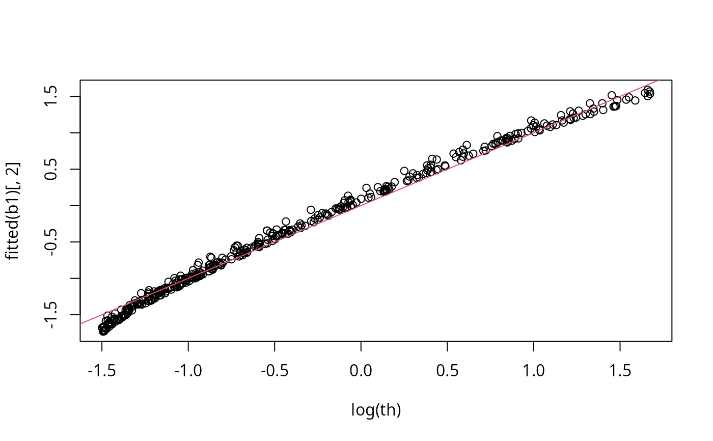
 plot(log(th),fitted(b1)[,2]);abline(0,1,col=2)