GAM ordered categorical family
ocat.RdFamily for use with gam or bam, implementing regression for ordered categorical data.
A linear predictor provides the expected value of a latent variable following a logistic distribution. The
probability of this latent variable lying between certain cut-points provides the probability of the ordered
categorical variable being of the corresponding category. The cut-points are estimated along side the model
smoothing parameters (using the same criterion). The observed categories are coded 1, 2, 3, ... up to the
number of categories.
ocat(theta=NULL,link="identity",R=NULL)Arguments
- theta
cut point parameter vector (dimension
R-2). If supplied and all positive, then taken to be the cut point increments (first cut point is fixed at -1). If any are negative then absolute values are taken as starting values for cutpoint increments.- link
The link function: only
"identity"allowed at present (possibly for ever).- R
the number of catergories.
Value
An object of class extended.family.
Details
Such cumulative threshold models are only identifiable up to an intercept, or one of the cut points.
Rather than remove the intercept, ocat simply sets the first cut point to -1. Use predict.gam with
type="response" to get the predicted probabilities in each category.
References
Wood, S.N., N. Pya and B. Saefken (2016), Smoothing parameter and model selection for general smooth models. Journal of the American Statistical Association 111, 1548-1575 doi:10.1080/01621459.2016.1180986
Examples
library(mgcv)
## Simulate some ordered categorical data...
set.seed(3);n<-400
dat <- gamSim(1,n=n)
#> Gu & Wahba 4 term additive model
dat$f <- dat$f - mean(dat$f)
alpha <- c(-Inf,-1,0,5,Inf)
R <- length(alpha)-1
y <- dat$f
u <- runif(n)
u <- dat$f + log(u/(1-u))
for (i in 1:R) {
y[u > alpha[i]&u <= alpha[i+1]] <- i
}
dat$y <- y
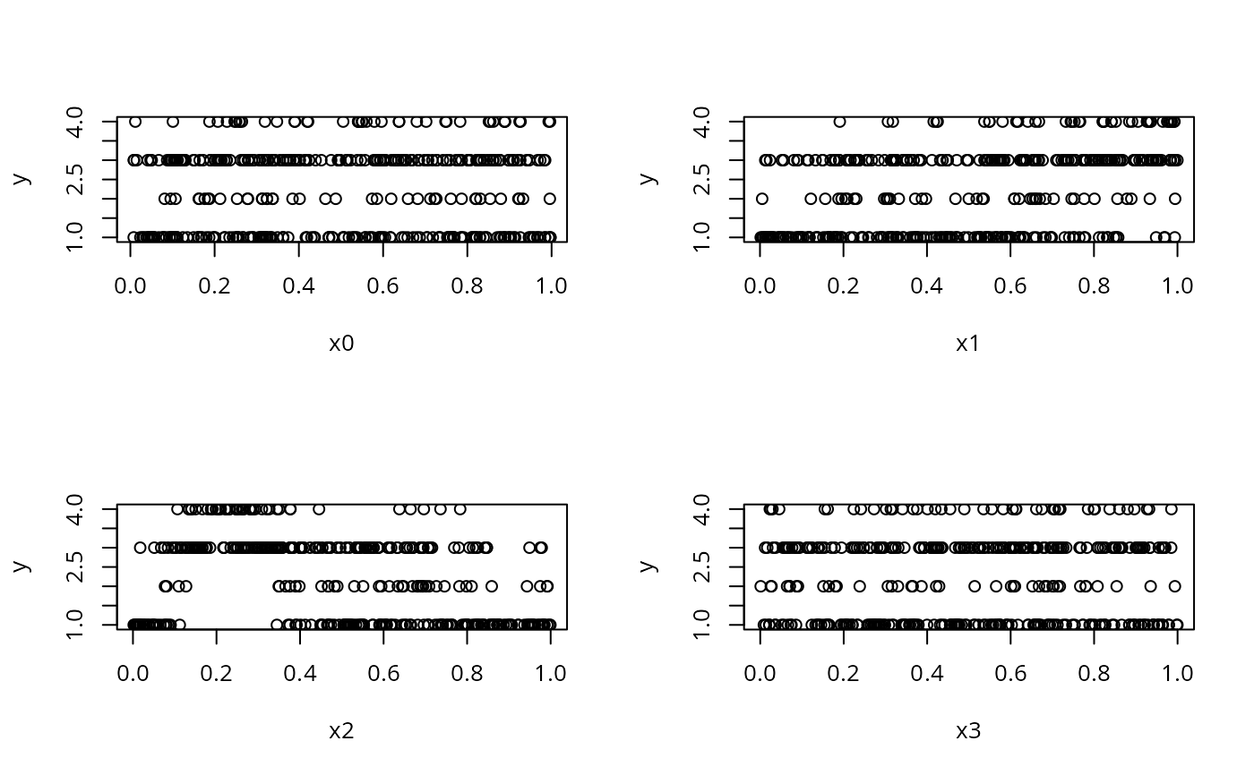
## plot the data...
par(mfrow=c(2,2))
with(dat,plot(x0,y));with(dat,plot(x1,y))
with(dat,plot(x2,y));with(dat,plot(x3,y))
 ## fit ocat model to data...
b <- gam(y~s(x0)+s(x1)+s(x2)+s(x3),family=ocat(R=R),data=dat)
b
#>
#> Family: Ordered Categorical(-1,0.07,5.15)
#> Link function: identity
#>
#> Formula:
#> y ~ s(x0) + s(x1) + s(x2) + s(x3)
#>
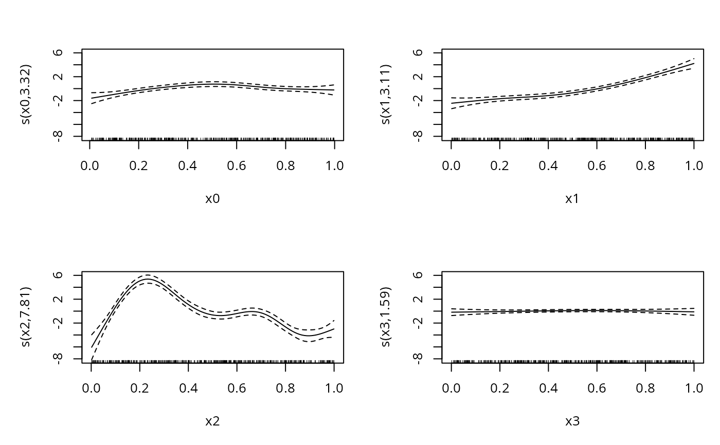
#> Estimated degrees of freedom:
#> 3.32 3.11 7.81 1.59 total = 16.84
#>
#> REML score: 283.8245
plot(b,pages=1)
## fit ocat model to data...
b <- gam(y~s(x0)+s(x1)+s(x2)+s(x3),family=ocat(R=R),data=dat)
b
#>
#> Family: Ordered Categorical(-1,0.07,5.15)
#> Link function: identity
#>
#> Formula:
#> y ~ s(x0) + s(x1) + s(x2) + s(x3)
#>
#> Estimated degrees of freedom:
#> 3.32 3.11 7.81 1.59 total = 16.84
#>
#> REML score: 283.8245
plot(b,pages=1)
 gam.check(b)
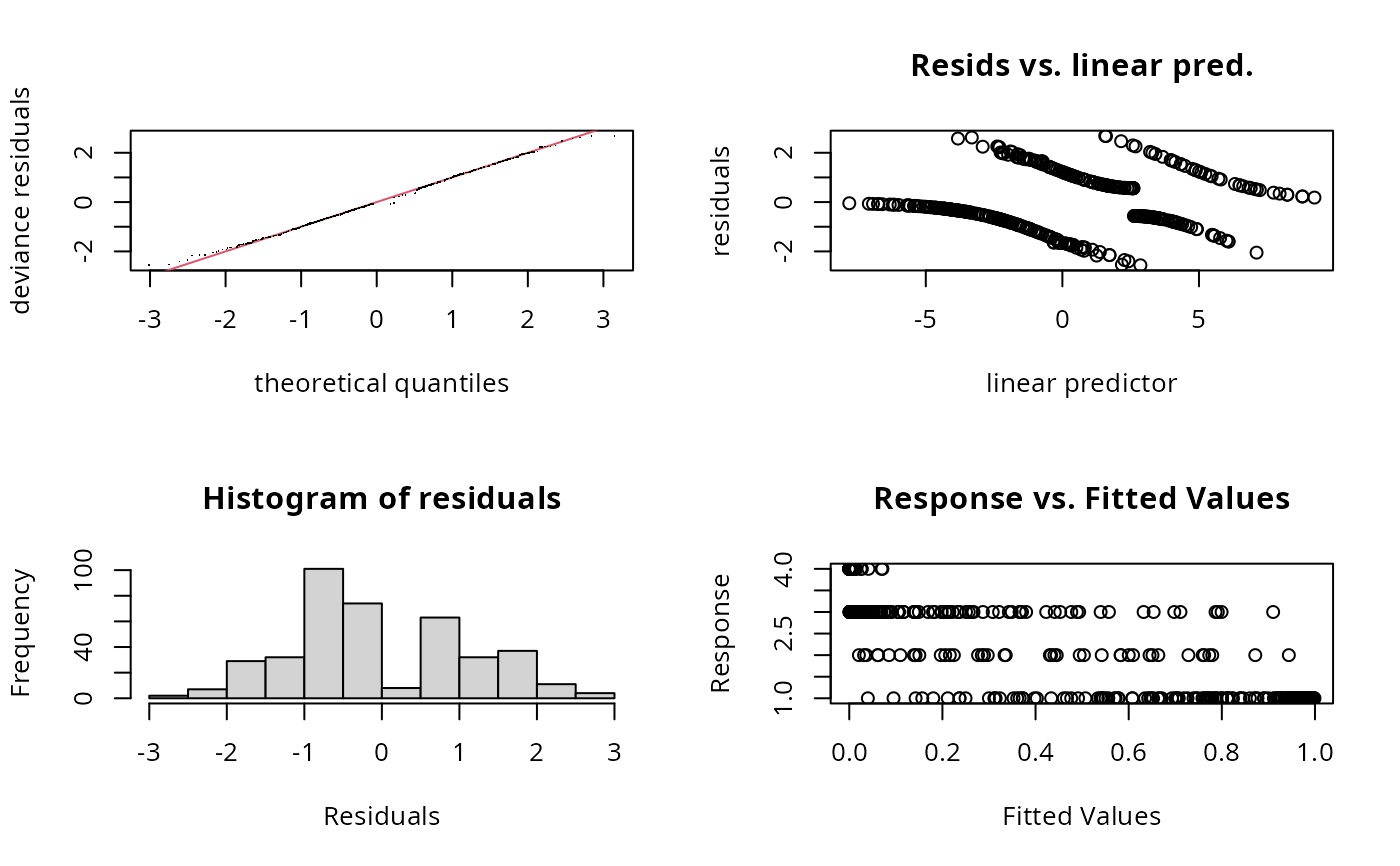 #>
#> Method: REML Optimizer: outer newton
#> full convergence after 5 iterations.
#> Gradient range [-4.800542e-06,4.973802e-08]
#> (score 283.8245 & scale 1).
#> Hessian positive definite, eigenvalue range [0.09977744,150.0804].
#> Model rank = 37 / 37
#>
#> Basis dimension (k) checking results. Low p-value (k-index<1) may
#> indicate that k is too low, especially if edf is close to k'.
#>
#> k' edf k-index p-value
#> s(x0) 9.00 3.32 0.94 0.14
#> s(x1) 9.00 3.11 1.06 0.90
#> s(x2) 9.00 7.81 0.95 0.12
#> s(x3) 9.00 1.59 0.97 0.28
summary(b)
#>
#> Family: Ordered Categorical(-1,0.07,5.15)
#> Link function: identity
#>
#> Formula:
#> y ~ s(x0) + s(x1) + s(x2) + s(x3)
#>
#> Parametric coefficients:
#> Estimate Std. Error z value Pr(>|z|)
#> (Intercept) 0.1221 0.1319 0.926 0.354
#>
#> Approximate significance of smooth terms:
#> edf Ref.df Chi.sq p-value
#> s(x0) 3.317 4.116 21.623 0.000264 ***
#> s(x1) 3.115 3.871 188.368 < 2e-16 ***
#> s(x2) 7.814 8.616 402.300 < 2e-16 ***
#> s(x3) 1.593 1.970 0.936 0.641757
#> ---
#> Signif. codes: 0 ‘***’ 0.001 ‘**’ 0.01 ‘*’ 0.05 ‘.’ 0.1 ‘ ’ 1
#>
#> Deviance explained = 57.6%
#> -REML = 283.82 Scale est. = 1 n = 400
b$family$getTheta(TRUE) ## the estimated cut points
#> [1] -1.00000000 0.07295739 5.14663505
## predict probabilities of being in each category
predict(b,dat[1:2,],type="response",se=TRUE)
#> $fit
#> [,1] [,2] [,3] [,4]
#> 1 0.99085777 0.005996704 0.003125774 0.0000197507
#> 2 0.06793525 0.107745442 0.795787468 0.0285318416
#>
#> $se.fit
#> [,1] [,2] [,3] [,4]
#> 1 0.006829264 0.00446533 0.002349044 1.488965e-05
#> 2 0.028948637 0.03725874 0.053535372 1.267200e-02
#>
#>
#> Method: REML Optimizer: outer newton
#> full convergence after 5 iterations.
#> Gradient range [-4.800542e-06,4.973802e-08]
#> (score 283.8245 & scale 1).
#> Hessian positive definite, eigenvalue range [0.09977744,150.0804].
#> Model rank = 37 / 37
#>
#> Basis dimension (k) checking results. Low p-value (k-index<1) may
#> indicate that k is too low, especially if edf is close to k'.
#>
#> k' edf k-index p-value
#> s(x0) 9.00 3.32 0.94 0.14
#> s(x1) 9.00 3.11 1.06 0.90
#> s(x2) 9.00 7.81 0.95 0.12
#> s(x3) 9.00 1.59 0.97 0.28
summary(b)
#>
#> Family: Ordered Categorical(-1,0.07,5.15)
#> Link function: identity
#>
#> Formula:
#> y ~ s(x0) + s(x1) + s(x2) + s(x3)
#>
#> Parametric coefficients:
#> Estimate Std. Error z value Pr(>|z|)
#> (Intercept) 0.1221 0.1319 0.926 0.354
#>
#> Approximate significance of smooth terms:
#> edf Ref.df Chi.sq p-value
#> s(x0) 3.317 4.116 21.623 0.000264 ***
#> s(x1) 3.115 3.871 188.368 < 2e-16 ***
#> s(x2) 7.814 8.616 402.300 < 2e-16 ***
#> s(x3) 1.593 1.970 0.936 0.641757
#> ---
#> Signif. codes: 0 ‘***’ 0.001 ‘**’ 0.01 ‘*’ 0.05 ‘.’ 0.1 ‘ ’ 1
#>
#> Deviance explained = 57.6%
#> -REML = 283.82 Scale est. = 1 n = 400
b$family$getTheta(TRUE) ## the estimated cut points
#> [1] -1.00000000 0.07295739 5.14663505
## predict probabilities of being in each category
predict(b,dat[1:2,],type="response",se=TRUE)
#> $fit
#> [,1] [,2] [,3] [,4]
#> 1 0.99085777 0.005996704 0.003125774 0.0000197507
#> 2 0.06793525 0.107745442 0.795787468 0.0285318416
#>
#> $se.fit
#> [,1] [,2] [,3] [,4]
#> 1 0.006829264 0.00446533 0.002349044 1.488965e-05
#> 2 0.028948637 0.03725874 0.053535372 1.267200e-02
#>