Random effects in GAMs
random.effects.RdThe smooth components of GAMs can be viewed as random effects for estimation purposes. This means that more conventional
random effects terms can be incorporated into GAMs in two ways. The first method converts all the smooths into fixed and random components
suitable for estimation by standard mixed modelling software. Once the GAM is in this form then conventional random effects are easily added,
and the whole model is estimated as a general mixed model. gamm and gamm4 from the gamm4 package operate in this way.
The second method represents the conventional random effects in a GAM in the same way that the smooths are represented — as penalized
regression terms. This method can be used with gam by making use of s(...,bs="re") terms in a model: see
smooth.construct.re.smooth.spec, for full details. The basic idea is that, e.g., s(x,z,g,bs="re") generates an i.i.d. Gaussian
random effect with model matrix given by model.matrix(~x:z:g-1) — in principle such terms can take any number of arguments. This simple
approach is sufficient for implementing a wide range of commonly used random effect structures. For example if g is a factor then
s(g,bs="re") produces a random coefficient for each level of g, with the random coefficients all modelled as i.i.d. normal. If g is a factor and x is numeric, then s(x,g,bs="re") produces an i.i.d. normal random slope relating the response to x for each level of g. If h is another factor then s(h,g,bs="re") produces the usual i.i.d. normal g - h interaction. Note that a rather useful approximate test for zero random effect is also implemented for such terms based on Wood (2013). If the precision
matrix is known to within a multiplicative constant, then this can be supplied via the xt argument of s. See smooth.construct.re.smooth.spec for details and example. Some models require differences between different levels of the same random effect: these can be implemented as described in linear.functional.terms.
Alternatively, but less straightforwardly, the paraPen argument to gam can be used:
see gam.models.
If smoothing parameter estimation is by ML or REML (e.g. gam(...,method="REML")) then this approach is
a completely conventional likelihood based treatment of random effects, using a full Laplace approximation to the (restricted) marginal likelihood. However note that MAP estimates of the model coefficients are returned. For the fixed effects in non-Gaussian cases, these are only approximately the MLEs (with the random effects integrated out), and the difference can be large in some circumstances.
gam can be slow for fitting models with large numbers of random effects, because it does not exploit the sparsity that is often a feature
of parametric random effects. It can not be used for models with more coefficients than data. However gam is often faster and more reliable
than gamm or gamm4, when the number of random effects is modest.
To facilitate the use of random effects with gam, gam.vcomp is a utility routine for converting
smoothing parameters to variance components. It also provides confidence intervals, if smoothness estimation is by ML or REML.
Note that treating random effects as smooths does not remove the usual problems associated with testing variance components for equality to zero: see summary.gam and anova.gam.
Note also that
See also
References
Wood, S.N. (2013) A simple test for random effects in regression models. Biometrika 100:1005-1010
Wood, S.N. (2011) Fast stable restricted maximum likelihood and marginal likelihood estimation of semiparametric generalized linear models. Journal of the Royal Statistical Society (B) 73(1):3-36
Wood, S.N. (2008) Fast stable direct fitting and smoothness selection for generalized additive models. Journal of the Royal Statistical Society (B) 70(3):495-518
Wood, S.N. (2006) Low rank scale invariant tensor product smooths for generalized additive mixed models. Biometrics 62(4):1025-1036
Examples
## see also examples for gam.models, gam.vcomp, gamm
## and smooth.construct.re.smooth.spec
## simple comparison of lme and gam
require(mgcv)
require(nlme)
b0 <- lme(travel~1,data=Rail,~1|Rail,method="REML")
b <- gam(travel~s(Rail,bs="re"),data=Rail,method="REML")
intervals(b0)
#> Approximate 95% confidence intervals
#>
#> Fixed effects:
#> lower est. upper
#> (Intercept) 44.33921 66.5 88.66079
#>
#> Random Effects:
#> Level: Rail
#> lower est. upper
#> sd((Intercept)) 13.27433 24.80547 46.35346
#>
#> Within-group standard error:
#> lower est. upper
#> 2.695005 4.020779 5.998752
gam.vcomp(b)
#>
#> Standard deviations and 0.95 confidence intervals:
#>
#> std.dev lower upper
#> s(Rail) 24.805465 13.274315 46.353510
#> scale 4.020779 2.695004 5.998753
#>
#> Rank: 2/2
#>
#> All smooth components:
#> [1] 24.80547
anova(b)
#>
#> Family: gaussian
#> Link function: identity
#>
#> Formula:
#> travel ~ s(Rail, bs = "re")
#>
#> Approximate significance of smooth terms:
#> edf Ref.df F p-value
#> s(Rail) 4.957 5.000 114.2 <2e-16
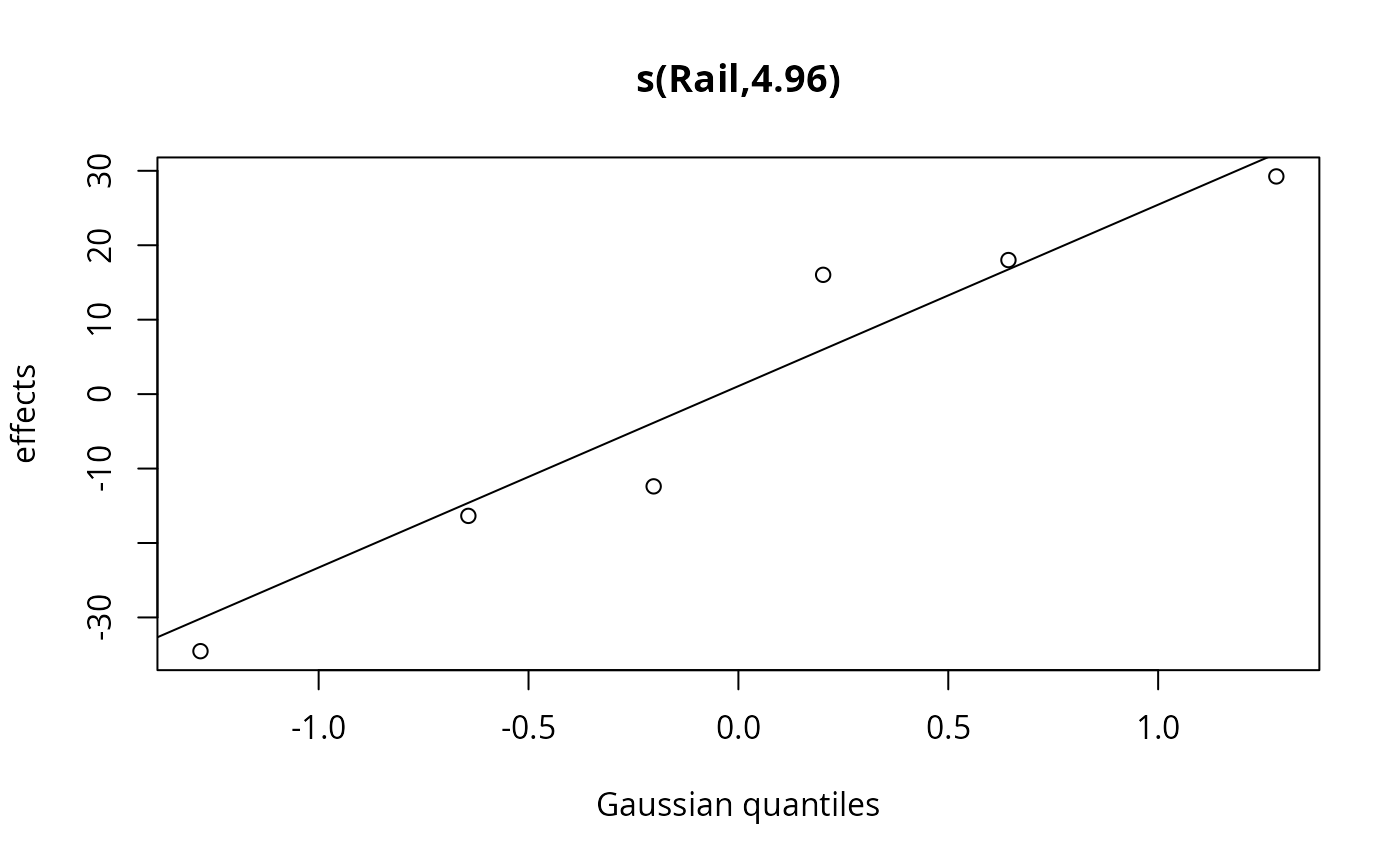
plot(b)
 ## simulate example...
dat <- gamSim(1,n=400,scale=2) ## simulate 4 term additive truth
#> Gu & Wahba 4 term additive model
fac <- sample(1:20,400,replace=TRUE)
b <- rnorm(20)*.5
dat$y <- dat$y + b[fac]
dat$fac <- as.factor(fac)
rm1 <- gam(y ~ s(fac,bs="re")+s(x0)+s(x1)+s(x2)+s(x3),data=dat,method="ML")
gam.vcomp(rm1)
#>
#> Standard deviations and 0.95 confidence intervals:
#>
#> std.dev lower upper
#> s(fac) 0.35254349 1.558099e-01 7.976828e-01
#> s(x0) 10.29847614 4.658579e+00 2.276630e+01
#> s(x1) 6.00267822 2.167535e+00 1.662356e+01
#> s(x2) 104.95219998 6.171205e+01 1.784897e+02
#> s(x3) 0.02732852 1.290189e-30 5.788670e+26
#> scale 1.98949805 1.850465e+00 2.138977e+00
#>
#> Rank: 6/6
#>
#> All smooth components:
#> [1] 0.35254349 10.29847614 6.00267822 104.95219998 0.02732852
fv0 <- predict(rm1,exclude="s(fac)") ## predictions setting r.e. to 0
fv1 <- predict(rm1) ## predictions setting r.e. to predicted values
## prediction setting r.e. to 0 and not having to provide 'fac'...
pd <- dat; pd$fac <- NULL
fv0 <- predict(rm1,pd,exclude="s(fac)",newdata.guaranteed=TRUE)
## Prediction with levels of fac not in fit data.
## The effect of the new factor levels (or any interaction involving them)
## is set to zero.
xx <- seq(0,1,length=10)
pd <- data.frame(x0=xx,x1=xx,x2=xx,x3=xx,fac=c(1:10,21:30))
fv <- predict(rm1,pd)
#> Warning: factor levels 21, 22, 23, 24, 25, 26, 27, 28, 29, 30 not in original fit
pd$fac <- NULL
fv0 <- predict(rm1,pd,exclude="s(fac)",newdata.guaranteed=TRUE)
## simulate example...
dat <- gamSim(1,n=400,scale=2) ## simulate 4 term additive truth
#> Gu & Wahba 4 term additive model
fac <- sample(1:20,400,replace=TRUE)
b <- rnorm(20)*.5
dat$y <- dat$y + b[fac]
dat$fac <- as.factor(fac)
rm1 <- gam(y ~ s(fac,bs="re")+s(x0)+s(x1)+s(x2)+s(x3),data=dat,method="ML")
gam.vcomp(rm1)
#>
#> Standard deviations and 0.95 confidence intervals:
#>
#> std.dev lower upper
#> s(fac) 0.35254349 1.558099e-01 7.976828e-01
#> s(x0) 10.29847614 4.658579e+00 2.276630e+01
#> s(x1) 6.00267822 2.167535e+00 1.662356e+01
#> s(x2) 104.95219998 6.171205e+01 1.784897e+02
#> s(x3) 0.02732852 1.290189e-30 5.788670e+26
#> scale 1.98949805 1.850465e+00 2.138977e+00
#>
#> Rank: 6/6
#>
#> All smooth components:
#> [1] 0.35254349 10.29847614 6.00267822 104.95219998 0.02732852
fv0 <- predict(rm1,exclude="s(fac)") ## predictions setting r.e. to 0
fv1 <- predict(rm1) ## predictions setting r.e. to predicted values
## prediction setting r.e. to 0 and not having to provide 'fac'...
pd <- dat; pd$fac <- NULL
fv0 <- predict(rm1,pd,exclude="s(fac)",newdata.guaranteed=TRUE)
## Prediction with levels of fac not in fit data.
## The effect of the new factor levels (or any interaction involving them)
## is set to zero.
xx <- seq(0,1,length=10)
pd <- data.frame(x0=xx,x1=xx,x2=xx,x3=xx,fac=c(1:10,21:30))
fv <- predict(rm1,pd)
#> Warning: factor levels 21, 22, 23, 24, 25, 26, 27, 28, 29, 30 not in original fit
pd$fac <- NULL
fv0 <- predict(rm1,pd,exclude="s(fac)",newdata.guaranteed=TRUE)