Psi / Chi / Wgt / Rho Functions for *M-Estimation
M.psi.RdCompute Psi / Chi / Wgt / Rho functions for M-estimation, i.e., including MM, etc. For definitions and details, please use the vignette “\(\psi\)-Functions Available in Robustbase”.
MrhoInf(x) computes \(\rho(\infty)\), i.e., the
normalizing or scaling constant for the transformation
from \(\rho(\cdot)\) to
\(\tilde\rho(\cdot)\), where the latter, aka as
\(\chi()\) fulfills \(\tilde\rho(\infty) = 1\)
which makes only sense for “redescending” psi functions, i.e.,
not for "huber".
Mwgt(x, *) computes \(\psi(x)/x\) (fast and numerically accurately).
Mpsi(x, cc, psi, deriv = 0)
Mchi(x, cc, psi, deriv = 0)
Mwgt(x, cc, psi)
MrhoInf(cc, psi)

.Mwgt.psi1(psi, cc = .Mpsi.tuning.default(psi))
.regularize.Mpsi(psi, redescending = TRUE)
Arguments
- x
numeric (“abscissa” values) vector, possibly with
attributessuch asdimornames, etc. These are preserved for theM*()functions (but not the.M()ones).- cc
numeric tuning constant, for some
psiof length \(> 1\).- psi
a string specifying the psi / chi / rho / wgt function; either
"huber", or one of the same possible specifiers as forpsiinlmrob.control, i.e. currently,"bisquare","lqq","welsh","optimal","hampel", or"ggw".- deriv
an integer, specifying the order of derivative to consider; particularly,
Mpsi(x, *, deriv = -1)is the principal function of \(\psi()\), typically denoted \(\rho()\) in the literature. For some psi functions, currently"huber","bisquare","hampel", and"lqq",deriv = 2is implemented, for the other psi's only \(d \in \{-1,0,1\}\)- redescending
logical indicating in
.regularize.Mpsi(psi,.)if thepsifunction is redescending.
Details
Theoretically, Mchi() would not be needed explicitly as it can be computed
from Mpsi() and MrhoInf(), namely, by
Mchi(x, *, deriv = d) == Mpsi(x, *, deriv = d-1) / MrhoInf(*)for \(d = 0, 1, 2\) (and ‘*’ containing par, psi, and
equality is in the sense of all.equal(x,y, tol) with a
small tol.
Similarly, Mwgt would not be needed strictly, as it could be
defined via Mpsi), but the explicit definition takes care of
0/0 and typically is of a more simple form.
For experts, there are slightly even faster versions,
.Mpsi(), .Mwgt(), etc.
.Mwgt.psi1() mainly a utility for nlrob(),
returns a function with similar semantics as
psi.hampel, psi.huber, or
psi.bisquare from package MASS. Namely,
a function with arguments (x, deriv=0), which for
deriv=0 computes Mwgt(x, cc, psi) and otherwise computes
Mpsi(x, cc, psi, deriv=deriv).
.Mpsi(), .Mchi(), .Mwgt(), and .MrhoInf() are
low-level versions of
Mpsi(), Mchi(), Mwgt(), and MrhoInf(), respectively,
and .psi2ipsi() provides the psi-function integer codes needed
for ipsi argument of the .M*() functions.
For psi = "ggw", the \(\rho()\) function has no closed
form and must be computed via numerical integration, apart from 6
special cases including the defaults, see the ‘Details’ in
help(.psi.ggw.findc).
.Mpsi.regularize() may (rarely) be used to regularize a psi function.
Value
a numeric vector of the same length as x, with corresponding
function (or derivative) values.
References
See the vignette about “\(\psi\)-Functions Available in Robustbase”.
See also
psiFunc and the psi_func class, both
of which provide considerably more on the R side, but are less
optimized for speed.
.Mpsi.tuning.defaults, etc, for tuning constants'
defaults forlmrob(), and .psi.ggw.findc()
utilities to construct such constants' vectors.
Examples
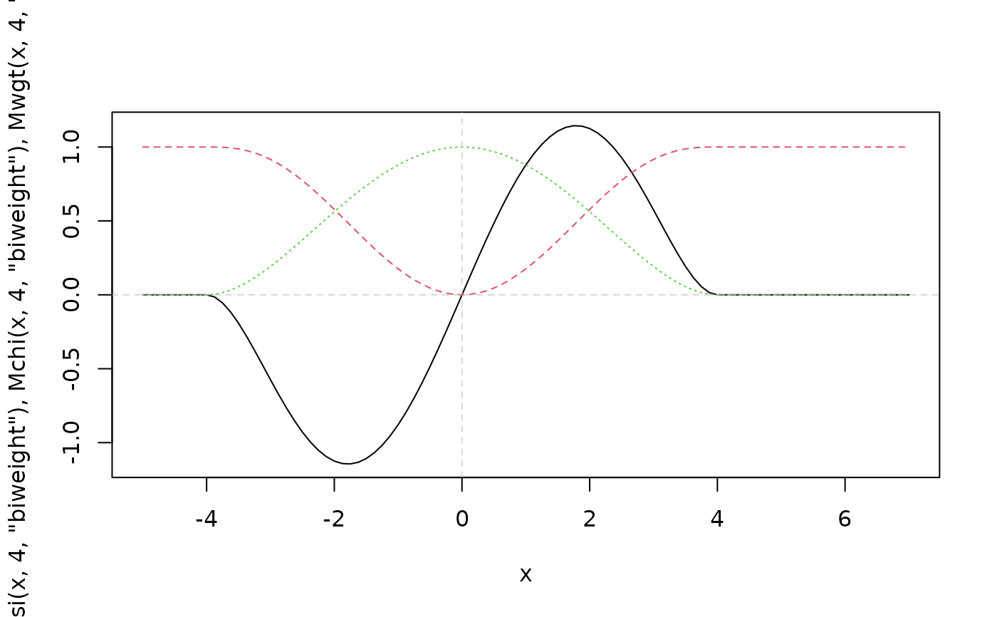
x <- seq(-5,7, by=1/8)
matplot(x, cbind(Mpsi(x, 4, "biweight"),
Mchi(x, 4, "biweight"),
Mwgt(x, 4, "biweight")), type = "l")
abline(h=0, v=0, lty=2, col=adjustcolor("gray", 0.6))
 hampelPsi
#> Hampel psi function (k1 = 1.487, k2 = 2.974, k3 = 5.948)
(ccHa <- hampelPsi @ xtras $ tuningP $ k)
#> [1] 1.486989 2.973978 5.947955
psHa <- hampelPsi@psi(x)
## using Mpsi():
Mp.Ha <- Mpsi(x, cc = ccHa, psi = "hampel")
stopifnot(all.equal(Mp.Ha, psHa, tolerance = 1e-15))
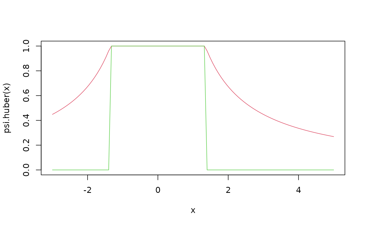
psi.huber <- .Mwgt.psi1("huber")
if(getRversion() >= "3.0.0")
stopifnot(identical(psi.huber, .Mwgt.psi1("huber", 1.345),
ignore.env=TRUE))
curve(psi.huber(x), -3, 5, col=2, ylim = 0:1)
curve(psi.huber(x, deriv=1), add=TRUE, col=3)
hampelPsi
#> Hampel psi function (k1 = 1.487, k2 = 2.974, k3 = 5.948)
(ccHa <- hampelPsi @ xtras $ tuningP $ k)
#> [1] 1.486989 2.973978 5.947955
psHa <- hampelPsi@psi(x)
## using Mpsi():
Mp.Ha <- Mpsi(x, cc = ccHa, psi = "hampel")
stopifnot(all.equal(Mp.Ha, psHa, tolerance = 1e-15))
psi.huber <- .Mwgt.psi1("huber")
if(getRversion() >= "3.0.0")
stopifnot(identical(psi.huber, .Mwgt.psi1("huber", 1.345),
ignore.env=TRUE))
curve(psi.huber(x), -3, 5, col=2, ylim = 0:1)
curve(psi.huber(x, deriv=1), add=TRUE, col=3)
 ## and show that this is indeed the same as MASS::psi.huber() :
x <- runif(256, -2,3)
stopifnot(all.equal(psi.huber(x), MASS::psi.huber(x)),
all.equal( psi.huber(x, deriv=1),
as.numeric(MASS::psi.huber(x, deriv=1))))
## and how to get MASS::psi.hampel():
psi.hampel <- .Mwgt.psi1("Hampel", c(2,4,8))
x <- runif(256, -4, 10)
stopifnot(all.equal(psi.hampel(x), MASS::psi.hampel(x)),
all.equal( psi.hampel(x, deriv=1),
as.numeric(MASS::psi.hampel(x, deriv=1))))
## "lqq" / "LQQ" and its tuning constants:
ctl0 <- lmrob.control(psi = "lqq", tuning.psi=c(-0.5, 1.5, 0.95, NA))
ctl <- lmrob.control(psi = "lqq", tuning.psi=c(-0.5, 1.5, 0.90, NA))
ctl0$tuning.psi ## keeps the vector _and_ has "constants" attribute:
#> [1] -0.50 1.50 0.95 NA
#> attr(,"constants")
#> [1] 1.4734061 0.9822707 1.5000000
## [1] -0.50 1.50 0.95 NA
## attr(,"constants")
## [1] 1.4734061 0.9822707 1.5000000
ctl$tuning.psi ## ditto:
#> [1] -0.5 1.5 0.9 NA
#> attr(,"constants")
#> [1] 1.213726 0.809151 1.500000
## [1] -0.5 1.5 0.9 NA \ .."constants" 1.213726 0.809151 1.500000
stopifnot(all.equal(Mpsi(0:2, cc = ctl$tuning.psi, psi = ctl$psi),
c(0, 0.977493, 1.1237), tol = 6e-6))
x <- seq(-4,8, by = 1/16)
## Show how you can use .Mpsi() equivalently to Mpsi()
stopifnot(all.equal( Mpsi(x, cc = ctl$tuning.psi, psi = ctl$psi),
.Mpsi(x, ccc = attr(ctl$tuning.psi, "constants"),
ipsi = .psi2ipsi("lqq"))))
stopifnot(all.equal( Mpsi(x, cc = ctl0$tuning.psi, psi = ctl0$psi, deriv=1),
.Mpsi(x, ccc = attr(ctl0$tuning.psi, "constants"),
ipsi = .psi2ipsi("lqq"), deriv=1)))
## M*() preserving attributes :
x <- matrix(x, 32, 8, dimnames=list(paste0("r",1:32), col=letters[1:8]))
#> Warning: data length [193] is not a sub-multiple or multiple of the number of rows [32]
comment(x) <- "a vector which is a matrix"
px <- Mpsi(x, cc = ccHa, psi = "hampel")
stopifnot(identical(attributes(x), attributes(px)))
## The "optimal" psi exists in two versions "in the litterature": ---
## Maronna et al. 2006, 5.9.1, p.144f:
psi.M2006 <- function(x, c = 0.013)
sign(x) * pmax(0, abs(x) - c/dnorm(abs(x)))
## and the other is the one in robustbase from 'robust': via Mpsi(.., "optimal")
## Here are both for 95% efficiency:
(c106 <- .Mpsi.tuning.default("optimal"))
#> [1] 1.060158
c1 <- curve(Mpsi(x, cc = c106, psi="optimal"), -5, 7, n=1001)
c2 <- curve(psi.M2006(x), add=TRUE, n=1001, col=adjustcolor(2,0.4), lwd=2)
abline(0,1, v=0, h=0, lty=3)
## and show that this is indeed the same as MASS::psi.huber() :
x <- runif(256, -2,3)
stopifnot(all.equal(psi.huber(x), MASS::psi.huber(x)),
all.equal( psi.huber(x, deriv=1),
as.numeric(MASS::psi.huber(x, deriv=1))))
## and how to get MASS::psi.hampel():
psi.hampel <- .Mwgt.psi1("Hampel", c(2,4,8))
x <- runif(256, -4, 10)
stopifnot(all.equal(psi.hampel(x), MASS::psi.hampel(x)),
all.equal( psi.hampel(x, deriv=1),
as.numeric(MASS::psi.hampel(x, deriv=1))))
## "lqq" / "LQQ" and its tuning constants:
ctl0 <- lmrob.control(psi = "lqq", tuning.psi=c(-0.5, 1.5, 0.95, NA))
ctl <- lmrob.control(psi = "lqq", tuning.psi=c(-0.5, 1.5, 0.90, NA))
ctl0$tuning.psi ## keeps the vector _and_ has "constants" attribute:
#> [1] -0.50 1.50 0.95 NA
#> attr(,"constants")
#> [1] 1.4734061 0.9822707 1.5000000
## [1] -0.50 1.50 0.95 NA
## attr(,"constants")
## [1] 1.4734061 0.9822707 1.5000000
ctl$tuning.psi ## ditto:
#> [1] -0.5 1.5 0.9 NA
#> attr(,"constants")
#> [1] 1.213726 0.809151 1.500000
## [1] -0.5 1.5 0.9 NA \ .."constants" 1.213726 0.809151 1.500000
stopifnot(all.equal(Mpsi(0:2, cc = ctl$tuning.psi, psi = ctl$psi),
c(0, 0.977493, 1.1237), tol = 6e-6))
x <- seq(-4,8, by = 1/16)
## Show how you can use .Mpsi() equivalently to Mpsi()
stopifnot(all.equal( Mpsi(x, cc = ctl$tuning.psi, psi = ctl$psi),
.Mpsi(x, ccc = attr(ctl$tuning.psi, "constants"),
ipsi = .psi2ipsi("lqq"))))
stopifnot(all.equal( Mpsi(x, cc = ctl0$tuning.psi, psi = ctl0$psi, deriv=1),
.Mpsi(x, ccc = attr(ctl0$tuning.psi, "constants"),
ipsi = .psi2ipsi("lqq"), deriv=1)))
## M*() preserving attributes :
x <- matrix(x, 32, 8, dimnames=list(paste0("r",1:32), col=letters[1:8]))
#> Warning: data length [193] is not a sub-multiple or multiple of the number of rows [32]
comment(x) <- "a vector which is a matrix"
px <- Mpsi(x, cc = ccHa, psi = "hampel")
stopifnot(identical(attributes(x), attributes(px)))
## The "optimal" psi exists in two versions "in the litterature": ---
## Maronna et al. 2006, 5.9.1, p.144f:
psi.M2006 <- function(x, c = 0.013)
sign(x) * pmax(0, abs(x) - c/dnorm(abs(x)))
## and the other is the one in robustbase from 'robust': via Mpsi(.., "optimal")
## Here are both for 95% efficiency:
(c106 <- .Mpsi.tuning.default("optimal"))
#> [1] 1.060158
c1 <- curve(Mpsi(x, cc = c106, psi="optimal"), -5, 7, n=1001)
c2 <- curve(psi.M2006(x), add=TRUE, n=1001, col=adjustcolor(2,0.4), lwd=2)
abline(0,1, v=0, h=0, lty=3)
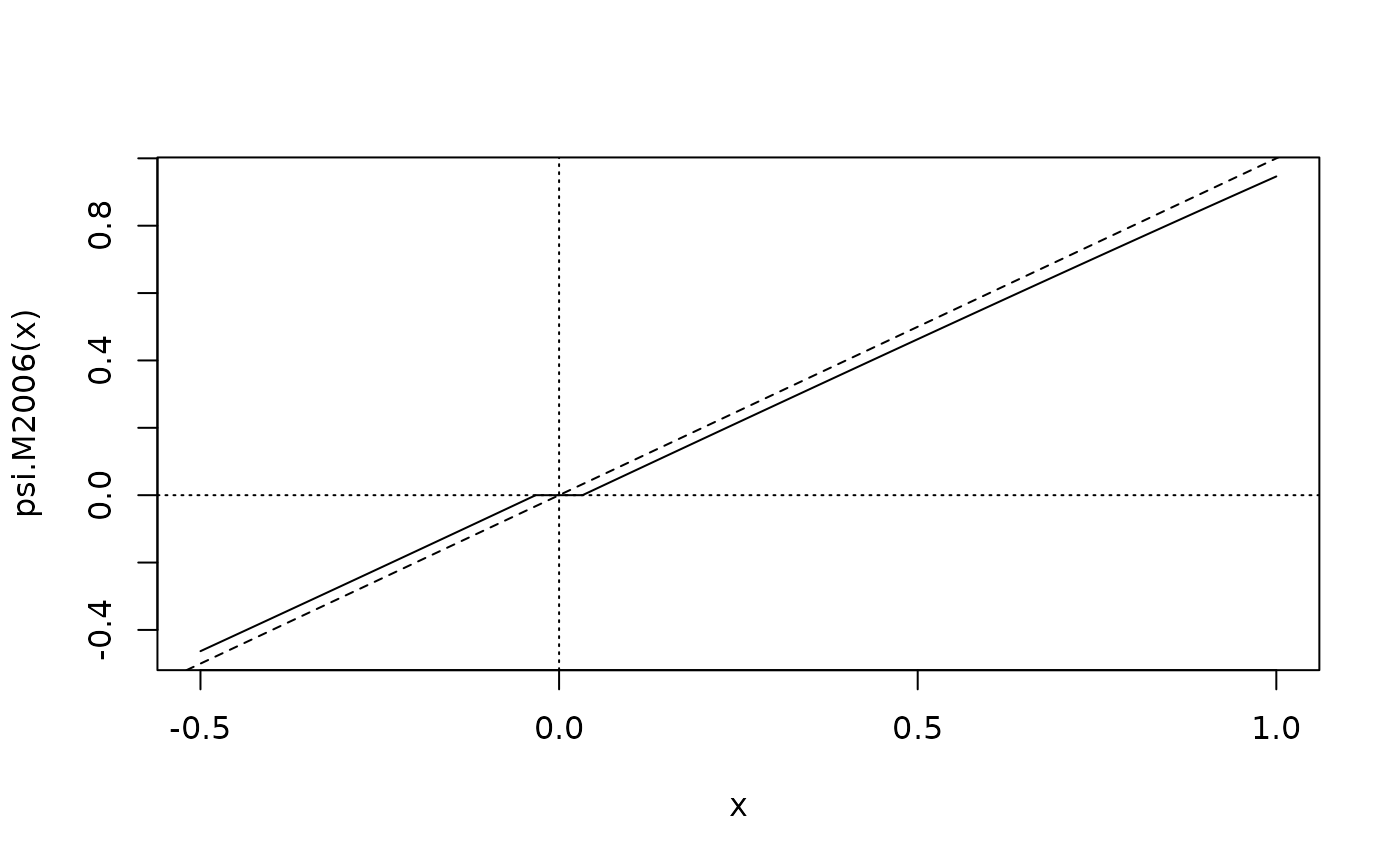
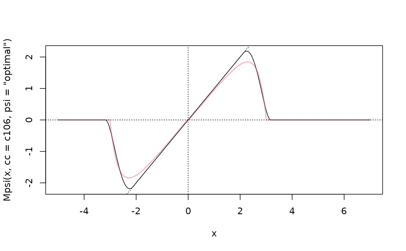 ## the two psi's are similar, but really quite different
## a zoom into Maronna et al's:
c3 <- curve(psi.M2006(x), -.5, 1, n=1001); abline(h=0,v=0, lty=3);abline(0,1, lty=2)
## the two psi's are similar, but really quite different
## a zoom into Maronna et al's:
c3 <- curve(psi.M2006(x), -.5, 1, n=1001); abline(h=0,v=0, lty=3);abline(0,1, lty=2)