Compute (Skewness-adjusted) Multivariate Outlyingness
adjOutlyingness.RdFor an \(n \times p\) data matrix (or data frame) x,
compute the “outlyingness” of all \(n\) observations.
Outlyingness here is a generalization of the Donoho-Stahel
outlyingness measure, where skewness is taken into account via the
medcouple, mc().
adjOutlyingness(x, ndir = 250, p.samp = p, clower = 4, cupper = 3,
                IQRtype = 7,
                alpha.cutoff = 0.75, coef = 1.5,
                qr.tol = 1e-12, keep.tol = 1e-12,
                only.outlyingness = FALSE, maxit.mult = max(100, p),
                trace.lev = 0,
                mcReflect = n <= 100, mcScale = TRUE, mcMaxit = 2*maxit.mult,
                mcEps1 = 1e-12, mcEps2 = 1e-15,
                mcTrace = max(0, trace.lev-1))
Arguments
- x
a numeric \(n \times p\)
matrixordata.frame, which must be of full rank \(p\).- ndir
positive integer specifying the number of directions that should be searched.
- p.samp
the sample size to use for finding good random directions, must be at least
p. The default,phad been hard coded previously.- clower, cupper
the constant to be used for the lower and upper tails, in order to transform the data towards symmetry. You can set
clower = 0, cupper = 0to get the non-adjusted, i.e., classical (“central” or “symmetric”) outlyingness. In that case,mc()is not used.- IQRtype
a number from
1:9, denoting type of empirical quantile computation for theIQR(). The default 7 corresponds toquantile's andIQR's default. MM has evidence thattype=6would be a bit more stable for small sample size.- alpha.cutoff
number in (0,1) specifying the quantiles \((\alpha, 1-\alpha)\) which determine the “outlier” cutoff. The default, using quartiles, corresponds to the definition of the medcouple (
mc), but there is no stringent reason for using the same alpha for the outlier cutoff.- coef
positive number specifying the factor with which the interquartile range (
IQR) is multiplied to determine ‘boxplot hinges’-like upper and lower bounds.- qr.tol
positive tolerance to be used for
qrandsolve.qrfor determining thendirdirections, each determined by a random sample of \(p\) (out of \(n\)) observations. Note that the default \(10^{-12}\) is rather small, andqr's default= 1e-7may be more appropriate.- keep.tol
positive tolerance to determine which of the sample direction should be kept, namely only those for which \(\|x\| \cdot \|B\|\) is larger than
keep.tol.- only.outlyingness
logical indicating if the final outlier determination should be skipped. In that case, a vector is returned, see ‘Value:’ below.
- maxit.mult
integer factor;
maxit <- maxit.mult * ndirwill determine the maximal number of direction searching iterations. May need to be increased for higher dimensional data, though increasingndirmay be more important.- trace.lev
an integer, if positive allows to monitor the direction search.
Note
If there are too many degrees of freedom for the projections, i.e., when
\(n \le 4p\), the current definition of adjusted outlyingness
is ill-posed, as one of the projections may lead to a denominator
(quartile difference) of zero, and hence formally an adjusted
outlyingness of infinity.
The current implementation avoids Inf results, but will return
seemingly random adjout values of around \(10^{14} -- 10^{15}\) which may
be completely misleading, see, e.g., the longley data example.
The result is random as it depends on the sample of
ndir directions chosen; specifically, to get sub samples the algorithm uses
sample.int(n, p.samp)
which from R version 3.6.0 depends on
RNGkind(*, sample.kind). Exact reproducibility of results
from R versions 3.5.3 and earlier, requires setting
RNGversion("3.5.0").
In any case, do use set.seed() yourself
for reproducibility!
Till Aug/Oct. 2014, the default values for clower and cupper were
accidentally reversed, and the signs inside exp(.) where swapped
in the (now corrected) two expressions
 tup <- Q3 + coef * IQR * exp(.... + clower * tmc * (tmc < 0))
 tlo <- Q1 - coef * IQR * exp(.... - cupper * tmc * (tmc < 0))
already in the code from Antwerpen (mcrsoft/adjoutlingness.R),
contrary to the published reference.
Further, the original algorithm had not been scale-equivariant in the direction construction, which has been amended in 2014-10 as well.
The results, including diagnosed outliers, therefore have changed, typically slightly, since robustbase version 0.92-0.
Details
FIXME: Details in the comment of the Matlab code; also in the reference(s).
The method as described can be useful as preprocessing in FASTICA (http://research.ics.aalto.fi/ica/fastica/ see also the R package fastICA.
Value
If only.outlyingness is true, a vector adjout,
otherwise, as by default, a list with components
- adjout
numeric of
length(n)giving the adjusted outlyingness of each observation.- cutoff
cutoff for “outlier” with respect to the adjusted outlyingnesses, and depending on
alpha.cutoff.- nonOut
logical of
length(n),TRUEwhen the corresponding observation is non-outlying with respect to the cutoff and the adjusted outlyingnesses.
References
Brys, G., Hubert, M., and Rousseeuw, P.J. (2005) A Robustification of Independent Component Analysis; Journal of Chemometrics, 19, 1–12.
Hubert, M., Van der Veeken, S. (2008) Outlier detection for skewed data; Journal of Chemometrics 22, 235–246; doi:10.1002/cem.1123 .
For the up-to-date reference, please consult https://wis.kuleuven.be/statdatascience/robust
Examples
## An Example with bad condition number and "border case" outliers
dim(longley) # 16 x 7 // set seed, as result is random :
#> [1] 16 7
set.seed(31)
ao1 <- adjOutlyingness(longley, mcScale=FALSE)
## which are outlying ?
which(!ao1$nonOut) ## for this seed, two: "1956", "1957"; (often: none)
#> named integer(0)
## For seeds 1:100, we observe (Linux 64b)
if(FALSE) {
adjO <- sapply(1:100, function(iSeed) {
set.seed(iSeed); adjOutlyingness(longley)$nonOut })
table(nrow(longley) - colSums(adjO))
}
## #{outl.}: 0 1 2 3
## #{cases}: 74 17 6 3
## An Example with outliers :
dim(hbk)
#> [1] 75 4
set.seed(1)
ao.hbk <- adjOutlyingness(hbk)
str(ao.hbk)
#> List of 7
#> $ adjout : num [1:75] 34.3 35.3 37.3 37.9 37.5 ...
#> $ iter : int 250
#> $ ndir.final : int 250
#> $ MCadjout : num 0.257
#> $ Qalph.adjout: Named num [1:2] 1.42 2.63
#> ..- attr(*, "names")= chr [1:2] "25%" "75%"
#> $ cutoff : Named num 6.55
#> ..- attr(*, "names")= chr "75%"
#> $ nonOut : logi [1:75] FALSE FALSE FALSE FALSE FALSE FALSE ...
hist(ao.hbk $adjout)## really two groups
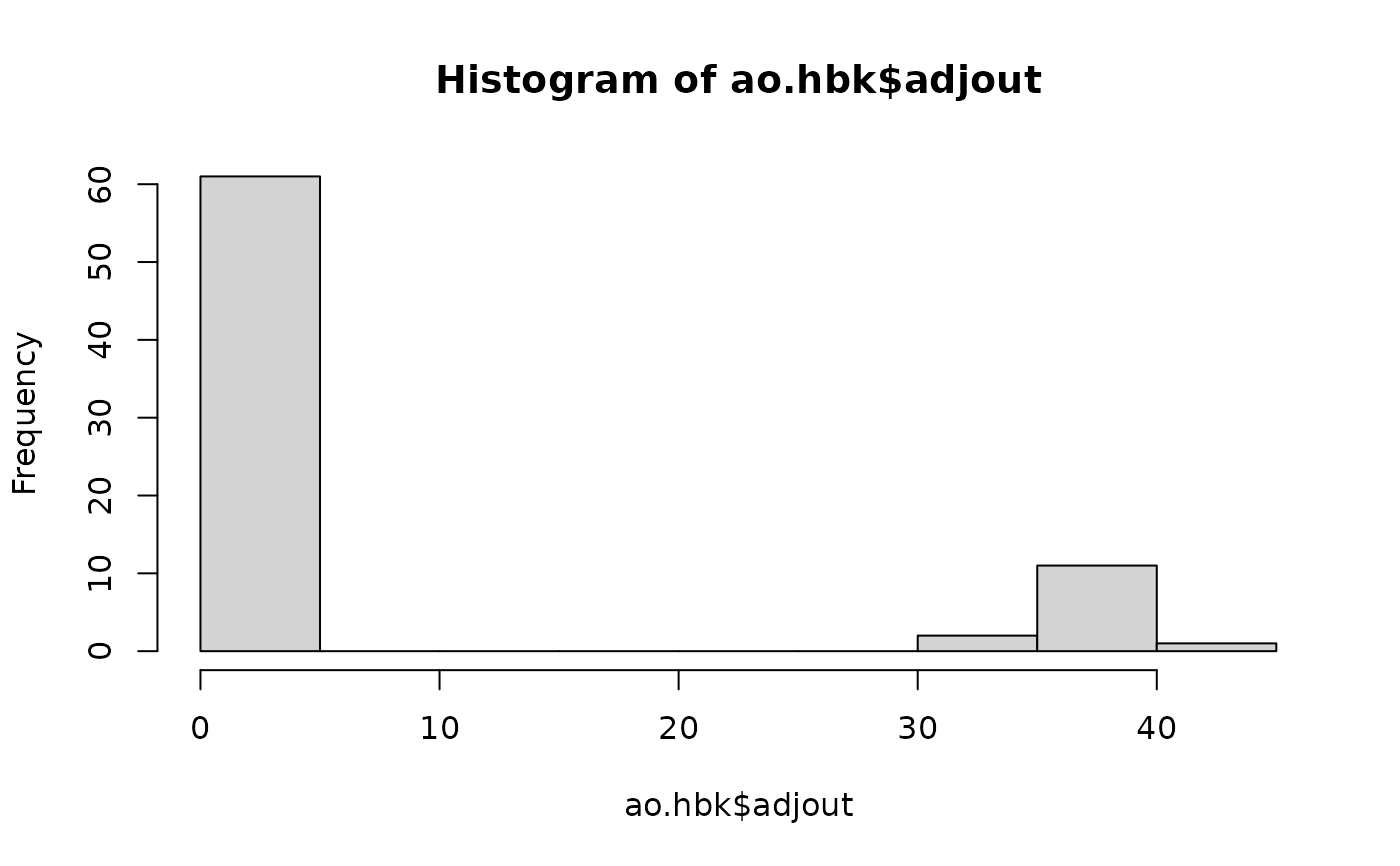 table(ao.hbk$nonOut)## 14 outliers, 61 non-outliers:
#>
#> FALSE TRUE
#> 14 61
## outliers are :
which(! ao.hbk$nonOut) # 1 .. 14 --- but not for all random seeds!
#> [1] 1 2 3 4 5 6 7 8 9 10 11 12 13 14
## here, they are(*) the same as found by (much faster) MCD:
## *) only "almost", since the 2023-05 change to covMcd()
cc <- covMcd(hbk)
table(cc = cc$mcd.wt, ao = ao.hbk$nonOut)# one differ..:
#> ao
#> cc FALSE TRUE
#> 0 14 1
#> 1 0 60
stopifnot(sum(cc$mcd.wt != ao.hbk$nonOut) <= 1)
## This is revealing: About 1--2 cases, where outliers are *not* == 1:14
## (2023: ~ 1/8 [sec] per call)
if(interactive()) {
for(i in 1:30) {
print(system.time(ao.hbk <- adjOutlyingness(hbk)))
if(!identical(iout <- which(!ao.hbk$nonOut), 1:14)) {
cat("Outliers:\n"); print(iout)
}
}
}
## "Central" outlyingness: *not* calling mc() anymore, since 2014-12-11:
trace(mc)
out <- capture.output(
oo <- adjOutlyingness(hbk, clower=0, cupper=0)
)
untrace(mc)
stopifnot(length(out) == 0)
## A rank-deficient case
T <- tcrossprod(data.matrix(toxicity))
try(adjOutlyingness(T, maxit. = 20, trace.lev = 2)) # fails and recommends:
#> it=1000: rank(qr(P ..)) = 10 < p = 38
#> it=2000: rank(qr(P ..)) = 10 < p = 38
#> it=3000: rank(qr(P ..)) = 10 < p = 38
#> it=4000: rank(qr(P ..)) = 10 < p = 38
#> Error in adjOutlyingness(T, maxit. = 20, trace.lev = 2) :
#> Matrix 'x' is not of full rank: rankM(x) = 10 < p = 38
#> Use fullRank(x) instead
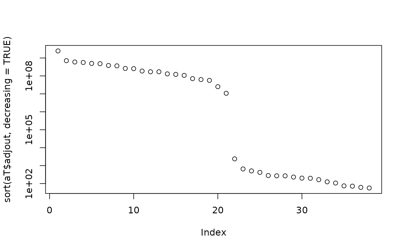
T. <- fullRank(T)
aT <- adjOutlyingness(T.)
plot(sort(aT$adjout, decreasing=TRUE), log="y")
table(ao.hbk$nonOut)## 14 outliers, 61 non-outliers:
#>
#> FALSE TRUE
#> 14 61
## outliers are :
which(! ao.hbk$nonOut) # 1 .. 14 --- but not for all random seeds!
#> [1] 1 2 3 4 5 6 7 8 9 10 11 12 13 14
## here, they are(*) the same as found by (much faster) MCD:
## *) only "almost", since the 2023-05 change to covMcd()
cc <- covMcd(hbk)
table(cc = cc$mcd.wt, ao = ao.hbk$nonOut)# one differ..:
#> ao
#> cc FALSE TRUE
#> 0 14 1
#> 1 0 60
stopifnot(sum(cc$mcd.wt != ao.hbk$nonOut) <= 1)
## This is revealing: About 1--2 cases, where outliers are *not* == 1:14
## (2023: ~ 1/8 [sec] per call)
if(interactive()) {
for(i in 1:30) {
print(system.time(ao.hbk <- adjOutlyingness(hbk)))
if(!identical(iout <- which(!ao.hbk$nonOut), 1:14)) {
cat("Outliers:\n"); print(iout)
}
}
}
## "Central" outlyingness: *not* calling mc() anymore, since 2014-12-11:
trace(mc)
out <- capture.output(
oo <- adjOutlyingness(hbk, clower=0, cupper=0)
)
untrace(mc)
stopifnot(length(out) == 0)
## A rank-deficient case
T <- tcrossprod(data.matrix(toxicity))
try(adjOutlyingness(T, maxit. = 20, trace.lev = 2)) # fails and recommends:
#> it=1000: rank(qr(P ..)) = 10 < p = 38
#> it=2000: rank(qr(P ..)) = 10 < p = 38
#> it=3000: rank(qr(P ..)) = 10 < p = 38
#> it=4000: rank(qr(P ..)) = 10 < p = 38
#> Error in adjOutlyingness(T, maxit. = 20, trace.lev = 2) :
#> Matrix 'x' is not of full rank: rankM(x) = 10 < p = 38
#> Use fullRank(x) instead
T. <- fullRank(T)
aT <- adjOutlyingness(T.)
plot(sort(aT$adjout, decreasing=TRUE), log="y")
 plot(T.[,9:10], col = (1:2)[1 + (aT$adjout > 10000)])
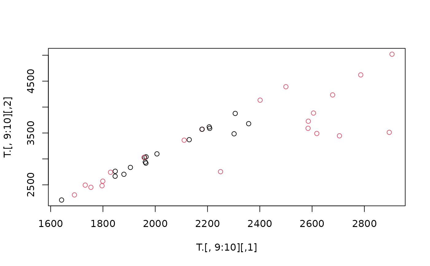 ## .. (not conclusive; directions are random, more 'ndir' makes a difference!)