Residuals of Robust Generalized Linear Model Fits

Compute residuals of a fitted glmrob model, i.e., robust generalized linear model fit.

# S3 method for class 'glmrob'
residuals(object,
          type = c("deviance", "pearson", "working",
                   "response", "partial"),
          ...)

Arguments

object

an object of class glmrob, typically the result of a call to glmrob.

type

the type of residuals which should be returned. The alternatives are: "deviance" (default), "pearson", "working", "response", and "partial".

...

further arguments passed to or from other methods.

Details

The references in glm define the types of residuals: Davison & Snell is a good reference for the usages of each.

The partial residuals are a matrix of working residuals, with each column formed by omitting a term from the model.

The residuals (S3) method (see methods) for glmrob models has been modeled to follow closely the method for classical (non-robust) glm fitted models. Possibly, see its documentation, i.e., residuals.glm, for further details.

See also

glmrob for computing object, anova.glmrob; the corresponding generic functions, summary.glmrob, coef, fitted, residuals.

References

See those for the classical GLM's, glm.

Examples

### -------- Gamma family -- data from example(glm) ---
clotting <- data.frame(
            u = c(5,10,15,20,30,40,60,80,100),
         lot1 = c(118,58,42,35,27,25,21,19,18),
         lot2 = c(69,35,26,21,18,16,13,12,12))
summary(cl <- glm   (lot1 ~ log(u), data=clotting, family=Gamma))
#> 
#> Call:
#> glm(formula = lot1 ~ log(u), family = Gamma, data = clotting)
#> 
#> Coefficients:
#>               Estimate Std. Error t value Pr(>|t|)    
#> (Intercept) -0.0165544  0.0009275  -17.85 4.28e-07 ***
#> log(u)       0.0153431  0.0004150   36.98 2.75e-09 ***
#> ---
#> Signif. codes:  0 ‘***’ 0.001 ‘**’ 0.01 ‘*’ 0.05 ‘.’ 0.1 ‘ ’ 1
#> 
#> (Dispersion parameter for Gamma family taken to be 0.002446059)
#> 
#>     Null deviance: 3.51283  on 8  degrees of freedom
#> Residual deviance: 0.01673  on 7  degrees of freedom
#> AIC: 37.99
#> 
#> Number of Fisher Scoring iterations: 3
#> 
summary(ro <- glmrob(lot1 ~ log(u), data=clotting, family=Gamma))
#> 
#> Call:  glmrob(formula = lot1 ~ log(u), family = Gamma, data = clotting) 
#> 
#> 
#> Coefficients:
#>               Estimate Std. Error z value Pr(>|z|)    
#> (Intercept) -0.0165260  0.0008369  -19.75   <2e-16 ***
#> log(u)       0.0153664  0.0003738   41.11   <2e-16 ***
#> ---
#> Signif. codes:  0 ‘***’ 0.001 ‘**’ 0.01 ‘*’ 0.05 ‘.’ 0.1 ‘ ’ 1
#> Robustness weights w.r * w.x: 
#> [1] 1.0000 0.6208 1.0000 1.0000 1.0000 1.0000 1.0000 1.0000 1.0000
#> 
#> Number of observations: 9 
#> Fitted by method ‘Mqle’  (in 3 iterations)
#> 
#> (Dispersion parameter for Gamma family taken to be 0.001869399)
#> 
#> No deviance values available 
#> Algorithmic parameters: 
#>    acc    tcc 
#> 0.0001 1.3450 
#> maxit 
#>    50 
#> test.acc 
#>   "coef" 
#> 
clotM5.high <- within(clotting, { lot1[5] <- 60 })
cl5.high <- glm   (lot1 ~ log(u), data=clotM5.high, family=Gamma)
ro5.high <- glmrob(lot1 ~ log(u), data=clotM5.high, family=Gamma)
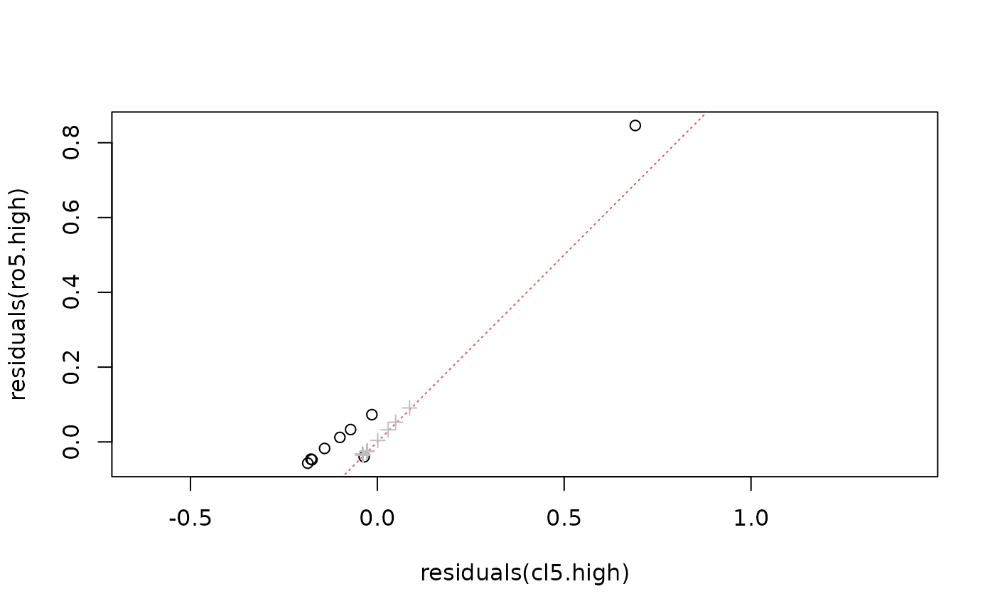
rr <- range(residuals(ro), residuals(cl), residuals(ro5.high))
plot(residuals(ro5.high) ~ residuals(cl5.high), xlim = rr, ylim = rr, asp = 1)
abline(0,1, col=2, lty=3)
points(residuals(ro) ~ residuals(cl), col = "gray", pch=3)


## Show all kinds of residuals:
r.types <- c("deviance", "pearson", "working", "response")
sapply(r.types, residuals, object = ro5.high)
#>      deviance     pearson     working   response
#> 1 -0.03981550 -0.03928883 -0.03928883 -4.8256777
#> 2  0.07296761  0.07475306  0.07475306  4.0341149
#> 3  0.03313416  0.03350112  0.03350112  1.3614374
#> 4  0.01211012  0.01215906  0.01215906  0.4204547
#> 5  0.84608494  1.09974648  1.09974648 31.4251217
#> 6 -0.01741507 -0.01731412 -0.01731412 -0.4404795
#> 7 -0.04768288 -0.04692803 -0.04692803 -1.0340127
#> 8 -0.05684730 -0.05577523 -0.05577523 -1.1223275
#> 9 -0.04597419 -0.04527236 -0.04527236 -0.8535445